Data/Model comparison

In oimodeler the oimSimulator class is the main class to do data/model comparison. In these section we will present:

• the basics use and functionalities of this class

• some details on how the simluated interferometric data are computed

• a description of the available plotting methods of the oimSimulator class

The code for this section is in SimulatingData.py

The basics of the simulator

To demonstrate the use of the oimSimulator class we will first use a single MIRCX observation of the binary star \(\beta\) Ari.

The oifits file of this observations can be found in the data directory of the oimodeler github website ( here).

We first get the path to the oifits file:

file = data_dir / "MIRCX_L2.2023Oct14._bet_Ari.MIRCX_IDL.nn.AVG10m.fits"

First, we need to build a model of a binary star where both of the components can be partly resolved. To do so, we use two uniform disks.

ud1 = oim.oimUD(d=1, f=0.8)
ud2 = oim.oimUD(d=0.8, f=0.2, x=5, y=15)
model = oim.oimModel([ud1, ud2])

We now create an oimSimulator object and feed it with the data and our model.

The data can either be:

• A previously created oimData.

• A list of previously opened astropy.io.fits.hdulist.

• A list of paths to the OIFITS files (list of strings).

sim = oim.oimSimulator(data=file, model=model)

If the data is given a filename or a list of filenames, the simulator automatically create an oimData instance containing the data as explained in the Loading & manipulating data section of this manual.

The loaded data can be directly accessed in the simulator using the data member variable. We can, for instance use the info to get the description of the data we have loaded into our simulator

sim.data.info()

════════════════════════════════════════════════════════════════════════════════
file 0: MIRCX_L2.2023Oct14._bet_Ari.MIRCX_IDL.nn.AVG10m.fits
────────────────────────────────────────────────────────────────────────────────
4)   OI_VIS  :       (nB,nλ) = (270, 15)     dataTypes = ['VISAMP', 'VISPHI']
5)   OI_VIS2 :       (nB,nλ) = (20, 15)      dataTypes = ['VIS2DATA']
6)   OI_T3   :       (nB,nλ) = (20, 15)      dataTypes = ['T3AMP', 'T3PHI']
════════════════════════════════════════════════════════════════════════════════

Here we see that our data contains one file with one instance of OI_VIS, OI_VIS2 and OI_T3 tables.

Similarly, we can access to our model within the simulator:

print(sim.model)

Model with
Uniform Disk: x=0.00 y=0.00 f=0.80 d=1.00
Uniform Disk: x=5.00 y=15.00 f=0.20 d=0.80

We can now simulate data using our model and the spatial coordinates of our loaded oifits files. This is done using the oimSimulator.compute method of the simulator instance.

This method have two boolean options:

• computeSimulatedData: compute the simulated data

• computeChi2: compute the :math:`chi^2`between the data and the model

sim.compute(computeChi2=True, computeSimulatedData=True)

The simulator will first call the oimModel.getComplexCoherentFlux method with optimized vectors of spatial, spectral and time coordinates.

If computeSimulatedData is True, the results of the oimModel.getComplexCoherentFlux is converted into a oimData instance accessible through the data member variable of the simulator.

sim.simulatedData.info()

════════════════════════════════════════════════════════════════════════════════
file 0: MIRCX_L2.2023Oct14._bet_Ari.MIRCX_IDL.nn.AVG10m.fits
────────────────────────────────────────────────────────────────────────────────
4)   OI_VIS  :       (nB,nλ) = (270, 15)     dataTypes = ['VISAMP', 'VISPHI']
5)   OI_VIS2 :       (nB,nλ) = (20, 15)      dataTypes = ['VIS2DATA']
6)   OI_T3   :       (nB,nλ) = (20, 15)      dataTypes = ['T3AMP', 'T3PHI']
════════════════════════════════════════════════════════════════════════════════

Or course, such instance have the same format (number of files, oi arrays, shape,…) as the original data.

Note

oimodeler can compute all data type from the OIFITS2 format.

The simulatedData can used to plot the data/model comparison. We this, we can used standard oimodeler plotting function or the oimSimulator.compute method fro mthe simulator. In that case, the user just need to pass the data types to be plotted, for instance, to plot the square visibility and closure phase:

fig0, ax0 = sim.plot(["VIS2DATA", "T3PHI"])

If the computeChi2 option is set to True, the user can retrieve the following quantities related to the \(\chi^2\) as member variables of the oimSimulator instance:

• chi2: the \(\chi^2\)

• chi2r: the \(\chi^2_r\) (i.e., the reduced \(\chi^2\))

• chi2List: a list of the residuals on all data and datatypes

• nelChi2: the number of data-points used to compute the \(\chi^2\)

pprint("Chi2r = {}".format(sim.chi2r))

... Chi2r = 2710.412886555833

Warning

By default the simulator uses all data types to compute the chi2. In the case of our ASPRO simulated data, this is OK as all datatypes are computed. But for most real interferometric instruments, some data type should be ignore. It is often the case of the closure-ampltiude (T3AMP). For some instruments like MATISSE, one should choose between using VISAMP or VIS2DATA.

We can force the \(\chi^2\) computation to only a subset of datatypes using the dataTypes option of oimSimulator.compute method. For instance, in the following we only compute the chi2r on the square visibliity and closure-phase.

sim.compute(computeChi2=True, dataTypes=["VIS2DATA","T3PHI"])
pprint(f"Chi2r = {sim.chi2r}")

... Chi2r = 232.12015864012497

We could now try to fit the model “by hand”, or by making a loop on some parameters and looking at the \(\chi^2_r\). But oimodeler implement various fitter class to perform automatic model fitting as described in Model fitting section.

Simulating data

Here, give a bit more details on how each of OIFITS2 compatible data type is computed from the complex coherent flux (CCF) return by the oimModel.getComplexCoherentFlux method. To learn more about the data vectorization and optimization in oimodeler go back to the Model fitting section.

In the table below is the complete list of OIFITS2 data type, their corresponding fits extension, data name, and additional keyword needed to disentangle between some quantities. The formula used to extract these quantities from the CCF is also given in the table.

OIFITS2 quantities

Quantity	Extension	name	keyword	formula
Square visibility	OI_VIS2	VIS2DATA		\(\bigg|\frac{CCF[u,v,\lambda,t]}{CCF[0,0,\lambda,t]}\bigg|^2\)
Absolute visibility	OI_VIS	VISAMP	AMPTYP= absolute	\(\bigg|\frac{CCF[u,v,\lambda,t]}{CCF[0,0,\lambda,t]}\bigg|\)
Differential visibility	OI_VIS	VISAMP	AMPTYP= differential	\(\bigg|\frac{CCF[u,v,\lambda,t]}{<CCF>_B}\bigg|\)
Correlated flux	OI_VIS	VISAMP	AMPTYP= correlated flux	\(\bigg|CCF[u,v,\lambda,t]\bigg|\)
Absolute phase	OI_VIS	VISPHI	PHITYP= absolute	\(angle\bigg(CCF[u,v,\lambda,t]\bigg)\)
Differential phase	OI_VIS	VISPHI	PHITYP= differential	\(angle\bigg(CCF[u,v,\lambda,t]<CCF^*>_B\bigg)\)
Triple product amplitude	OI_T3	T3AMP		\(\bigg|TP[u1,u2,u3,v1,v2,v3,\lambda,t]\bigg|\)
Closure phase	OI_T3	T3PHI		\(angle\bigg(TP[u1,u2,u3,v1,v2,v3,\lambda,t]\bigg)\)
Flux	OI_FLUX	FLUXDATA		\(CCF[0,0,\lambda,t]\)

TP is the triple product :

\[TP = \frac{CCF[u1,v1,\lambda,t] \cdot CCF[u2,v2,\lambda,t] \cdot CCF^*[u3,v3,\lambda,t]}{CF[0,0,\lambda,t]}\]

Where u1,u2,u3 and v1,v2,v3 are the (u,v) coordinates of the three baselines used to compute the triple product, closure phase and amplitude. The term \(<CCF>_B\) is the per baseline average of the CCF used to compute differential visibility and phase.

The \(chi^2\) computation

Plotting methods

Currently, three plotting methods are implemented in the oimSimulator class for direct data/model comparison.

In the previous section we already described the plot that can be used to plot any OIFITS2 quantities as the function of the spatial frequency.

fig0, ax0 = sim.plot(["VIS2DATA", "T3PHI"])

One can also produce per baseline plot as a function of the wavelength using the plotWlTemplate method.

fig1 = sim.plotWlTemplate([["VIS2DATA"],["T3PHI"]],xunit="micron",figsize=(22,3))
fig1.set_legends(0.5,0.8,"$BASELINE$",["VIS2DATA","T3PHI"],fontsize=10,ha="center")

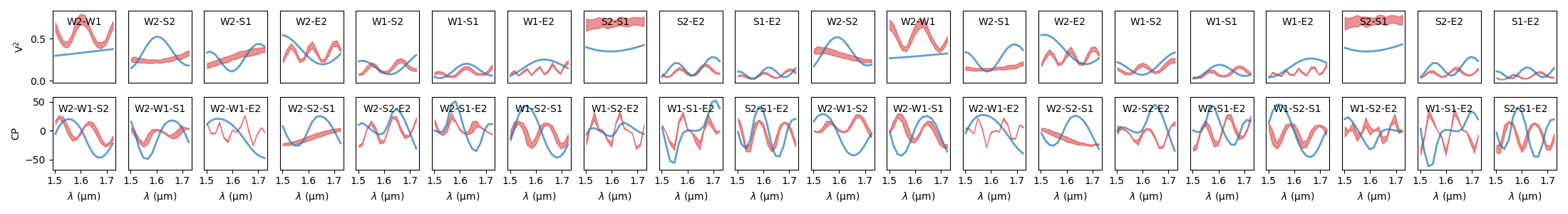
This method uses the oimWlTemplatePlots class as described more in details in the Plotting data section.

Such plot are very useful to plot high spectral resolution observation center on atomic lines such as for the Be star \(alpha\) Col VLTI/AMBER observation and modelling with a rotating disk model as described in the examples section.

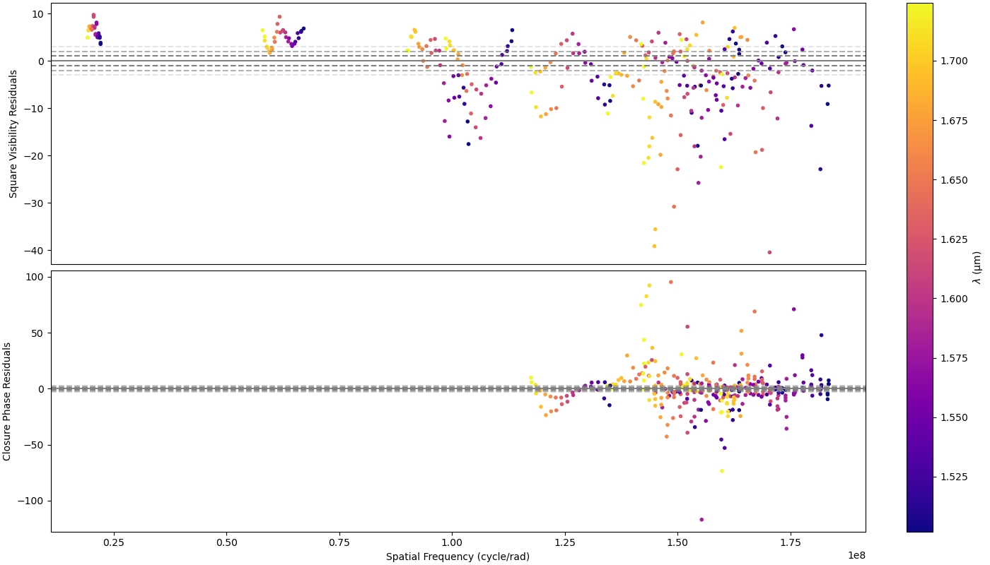
Finally, residuals can be plotted using the plot_residuals method.

fig2, ax2 = sim.plotResiduals(["VIS2DATA", "T3PHI"])