Loading & manipulating data
Interferometric data from all modern optical-infrared interferometric instruments are stored in FITS files following the OIFITS2 (Optical Interferometry FITS) standard defined in Duvert et al. (2017).
In oimodeler optical-interferometry data are stored in an oimData object. This object uses astropy.io.fits , the standard module to
load, save and manipulated FITS files.
Non-interferometric photometric or spectroscopic data can be added to an oimData object using the oimFluxData class.
Finally data can be filtered using the oimDataFilter class.
Interferometric data
This complete code corresponding to this section is available in InterferometricData.py
In oimodeler, data are stored in a oimData object. Other modules that requires access to data such as the oimSimulator and
oimFitter are all working with an instance of oimData.
The initialisation method of the oimData class allows to pass either a filename (in standard string or pathlib.Path), a list of filenames, a hdulist or a list of hdulist.
filenames = list(data_dir.glob("*.fits"))
data = oim.oimData(filenames)
Data in astropy format
The OIFITS data stored as a list of astropy.io.fits.hdulist can be accessed using the oimData.data attribute of the oimData object.
data.data
[[<astropy.io.fits.hdu.image.PrimaryHDU object at 0x0000017847722D10>, <astropy.io.fits.hdu.table.BinTableHDU object at 0x0000017847677490>, <astropy.io.fits.hdu.table.BinTableHDU object at 0x000001784767F6D0>, <astropy.io.fits.hdu.table.BinTableHDU object at 0x0000017847677DD0>, <astropy.io.fits.hdu.table.BinTableHDU object at 0x0000017847689AD0>, <astropy.io.fits.hdu.table.BinTableHDU object at 0x0000017847697D10>, <astropy.io.fits.hdu.table.BinTableHDU object at 0x0000017847689950>, <astropy.io.fits.hdu.table.BinTableHDU object at 0x0000017847573210>],
 [<astropy.io.fits.hdu.image.PrimaryHDU object at 0x000001784783BCD0>, <astropy.io.fits.hdu.table.BinTableHDU object at 0x0000017847689310>, <astropy.io.fits.hdu.table.BinTableHDU object at 0x000001784755A410>, <astropy.io.fits.hdu.table.BinTableHDU object at 0x0000017847554E10>, <astropy.io.fits.hdu.table.BinTableHDU object at 0x00000178475571D0>, <astropy.io.fits.hdu.table.BinTableHDU object at 0x000001784754BC10>, <astropy.io.fits.hdu.table.BinTableHDU object at 0x00000178475385D0>, <astropy.io.fits.hdu.table.BinTableHDU object at 0x0000017847556690>],
 [<astropy.io.fits.hdu.image.PrimaryHDU object at 0x00000178476BC710>, <astropy.io.fits.hdu.table.BinTableHDU object at 0x000001784752E3D0>, <astropy.io.fits.hdu.table.BinTableHDU object at 0x0000017847522410>, <astropy.io.fits.hdu.table.BinTableHDU object at 0x00000178474B8E10>, <astropy.io.fits.hdu.table.BinTableHDU object at 0x000001784752CE90>, <astropy.io.fits.hdu.table.BinTableHDU object at 0x00000178474C58D0>, <astropy.io.fits.hdu.table.BinTableHDU object at 0x00000178474C4450>, <astropy.io.fits.hdu.table.BinTableHDU object at 0x00000178474D4E10>]]
In this example, we loaded 3 oifits files so that our data variable is a list of three hdulist.
len(data.data)
3
We can have more readable informations calling the oimData.info method.
data.info()
════════════════════════════════════════════════════════════════════════════════
file 0: 2018-12-07T063809_HD45677_A0B2D0C1_IR-LM_LOW_Chop_cal_oifits_0.fits
────────────────────────────────────────────────────────────────────────────────
4)   OI_VIS2 :       (nB,nλ) = (6, 64)       dataTypes = ['VIS2DATA']
5)   OI_T3   :       (nB,nλ) = (4, 64)       dataTypes = ['T3PHI']
6)   OI_VIS  :       (nB,nλ) = (6, 64)       dataTypes = ['VISAMP', 'VISPHI']
7)   OI_FLUX :       (nB,nλ) = (1, 64)       dataTypes = ['FLUXDATA']
════════════════════════════════════════════════════════════════════════════════
file 1: 2018-12-07T063809_HD45677_A0B2D0C1_IR-LM_LOW_Chop_cal_oifits_0.fits
────────────────────────────────────────────────────────────────────────────────
4)   OI_VIS2 :       (nB,nλ) = (6, 64)       dataTypes = ['VIS2DATA']
5)   OI_T3   :       (nB,nλ) = (4, 64)       dataTypes = ['T3PHI']
6)   OI_VIS  :       (nB,nλ) = (6, 64)       dataTypes = ['VISAMP', 'VISPHI']
7)   OI_FLUX :       (nB,nλ) = (1, 64)       dataTypes = ['FLUXDATA']
════════════════════════════════════════════════════════════════════════════════
file 2: 2018-12-07T063809_HD45677_A0B2D0C1_IR-LM_LOW_Chop_cal_oifits_0.fits
────────────────────────────────────────────────────────────────────────────────
4)   OI_VIS2 :       (nB,nλ) = (6, 64)       dataTypes = ['VIS2DATA']
5)   OI_T3   :       (nB,nλ) = (4, 64)       dataTypes = ['T3PHI']
6)   OI_VIS  :       (nB,nλ) = (6, 64)       dataTypes = ['VISAMP', 'VISPHI']
7)   OI_FLUX :       (nB,nλ) = (1, 64)       dataTypes = ['FLUXDATA']
════════════════════════════════════════════════════════════════════════════════
In our case the OIFITS files contains the data extension OI_VIS2, OI_VIS, OI_T3 and OI_FLUX.
For each element of the list, we can call the info method of
the hdulist. class which lists all
extensions and gives some basics infos on what they contain.
data.data[0].info()
Filename: C:travailGitHuboimodelerdataFSCMa_MATISSE2018-12-07T063809_HD45677_A0B2D0C1_IR-LM_LOW_Chop_cal_oifits_0.fits
No.    Name      Ver    Type      Cards   Dimensions   Format
  0  PRIMARY       1 PrimaryHDU    1330   ()
  1  OI_TARGET     1 BinTableHDU     60   1R x 18C   [1I, 7A, 1D, 1D, 1E, 1D, 1D, 1D, 8A, 8A, 1D, 1D, 1D, 1D, 1E, 1E, 7A, 3A]
  2  OI_ARRAY      1 BinTableHDU     35   4R x 7C   [3A, 2A, 1I, 1E, 3D, 1D, 6A]
  3  OI_WAVELENGTH    1 BinTableHDU     20   64R x 2C   ['1E', '1E']
  4  OI_VIS2       1 BinTableHDU     41   6R x 10C   ['1I', '1D', '1D', '1D', '64D', '64D', '1D', '1D', '2I', '64L']
  5  OI_T3         1 BinTableHDU     53   4R x 14C   ['1I', '1D', '1D', '1D', '64D', '64D', '64D', '64D', '1D', '1D', '1D', '1D', '3I', '64L']
  6  OI_VIS        1 BinTableHDU     49   6R x 12C   ['1I', '1D', '1D', '1D', '64D', '64D', '64D', '64D', '1D', '1D', '2I', '64L']
  7  OI_FLUX       1 BinTableHDU     37   1R x 8C   ['I', 'D', 'D', 'D', '64D', '64D', 'I', '64L']
If needed, the user can access and modify the data directly.
For instance the following code double the errors on the VIS2DATA from the last OIFITS file:
data.data[2]["OI_VIS2"].data["VIS2ERR"]*= 2
Optimized data
In order to reduce the computation time when simulating data during model fitting, the oim:func:oimData.data <oimodeler.oimData.oimData> class also contain the data coordinates as single vectors and the logic to pass from optimized data (in a single vector) to unoptimized form (as a list of hdulist) as more complex structures (stored as lists of lists)
The data coordinates are stored in the following vectors:
The u-axis of the spatial frequencies
data.vect_uThe v-axis of the spatial frequencies
data.vect_vThe wavelength
data.vect_wlThe time (as MJD) data
data.vect_mjd
Let’s print their shape for our example:
print(data.vect_u.shape)
print(data.vect_v.shape)
print(data.vect_wl.shape)
print(data.vect_mjd.shape)
(5376,)
(5376,)
(5376,)
(5376,)
They contains all the coordinates of all the baselines at all wavelengths plus some zeros spatial frequencies data (used to computes flux and normaized visiblity).
On the other hand, to pass from the optimized data to unoptimized data are stored
in members called struct_XXXX. For instance, in the followin we print the
structures containing :
the number of baselines (including zero-frequency ones)
the number of wavelengths
the name of the extension
a code specifying which data type to compute: VIS2DATA, T3PHI, VIPHI (asbolute or differential) …
print(data.struct_nB)
print(data.struct_nwl)
print(data.struct_arrType)
print(data.struct_dataType)
[[7, 13, 7, 1], [7, 13, 7, 1], [7, 13, 7, 1]]
[[64, 64, 64, 64], [64, 64, 64, 64], [64, 64, 64, 64]]
[['OI_VIS2', 'OI_T3', 'OI_VIS', 'OI_FLUX'], ['OI_VIS2', 'OI_T3', 'OI_VIS', 'OI_FLUX'],
['OI_VIS2', 'OI_T3', 'OI_VIS', 'OI_FLUX']]
[[<oimDataType.VIS2DATA: 1>, <oimDataType.T3PHI: 128>, <oimDataType.VISAMP_ABS|VISPHI_DIF: 34>, <oimDataType.FLUXDATA: 256>],
[<oimDataType.VIS2DATA: 1>, <oimDataType.T3PHI: 128>, <oimDataType.VISAMP_ABS|VISPHI_DIF: 34>, <oimDataType.FLUXDATA: 256>],
[<oimDataType.VIS2DATA: 1>, <oimDataType.T3PHI: 128>, <oimDataType.VISAMP_ABS|VISPHI_DIF: 34>, <oimDataType.FLUXDATA: 256>]]
Note
The step of creating the optimized vectors and structures is done automatically
when creating or updating an oimData object. However if you modify the data
manually as shown above, you should call the
oimData.prepareData method.
The oimData object also contains two methods to plot :
oimData.uvplot: the (u,v) plan coverageoimData.plot: any data type (VIS2DATA, VISPHI …)
as a function of the spatial frequency, baseline length, position angle, or wavelength.
figuv, axuv = data.uvplot(color="byConfiguration")

figdata,axdata =  data.plot("SPAFREQ",["VIS2DATA","T3PHI"],cname="EFF_WAVE",
                           cunit="micron",errorbar=True,xunit="cycle/mas")
axdata[0].set_yscale("log")


- These pltting methods are based on the
uvplot and
oiplotmethods of theomiAxesclass. See the plotting section for details and option in plotting oifits data with oimodeler.
Data Filtering
This complete code corresponding to this section is available in DataFiltering.py
Data filtering can be performed on oimData
instances using the many filters that derived from the abstract
oimDataFilterComponent
The available data filters
Here is the compherensive list of filters implemented in oimodeler
Filter Name |
Short description |
Class Keywords |
|---|---|---|
oimDataFilterComponent |
This is the class from which all filters derived |
targets, arr |
oimRemoveArrayFilter |
Removing arrays by type: OI_VIS2, OI_T3… |
targets, arr |
oimRemoveInsnameFilter |
Remove array by insname |
targets, arr, insname |
oimWavelengthRangeFilter |
Cutting wavelength range(s) |
targets, arr, wlRange, addCut, method |
oimDataTypeFilter |
Filtering by datatype(s) : VIS2DATA, VISAMP… |
targets, arr, dataType |
oimKeepDataType |
Keep atatype that are listed: VIS2DATA, VISAMP… |
targets, arr, dataType, removeArrIfPossible |
oimWavelengthShiftFilter |
Shifting wavelength table |
targets, arr, wlShift |
oimWavelengthSmoothingFilter |
Spectral smoothing |
targets, arr, smoothPix, normalizeError |
oimWavelengthBinningFilter |
Spectral Binning |
targets, arr, bin, binGrid, normalizeError |
oimWavelengthIntpBinFilter |
Binning to wavelength grid with interpolation at window edges. |
targets, arr, binGrid, binWindow, resetFlags, averageError, spectralChannels |
oimFlagWithExpressionFilter |
Flagging based on boolean expressions |
targets, arr, expr, keepOldFlag |
oimKeepBaselinesFilter |
Selection based on baseline name(s) |
targets, arr, baselines, keepOldFlag |
oimRemoveBaselinesFilter |
Selection based on baseline name(s) |
targets, arr, baselines, keepOldFlag |
oimKeepTelescopesFilter |
Selection based on telescope name(s) |
targets, arr, telescopes, keepOldFlag |
oimRemoveTelescopesFilter |
Selection based on telescope name(s) |
targets, arr, telescopes, keepOldFlag |
oimResetFlags |
Set all the flags to False |
targets, arr |
oimDiffErrFilter |
Compute differential error from std inside or outside a range |
targets, arr, ranges, rangeType, excludeRange, dataType |
oimSetMinErrFilter |
Set minimum error on data in % for vis ans deg for phases |
targets, arr, values, dataType |
Applying filters to oimData
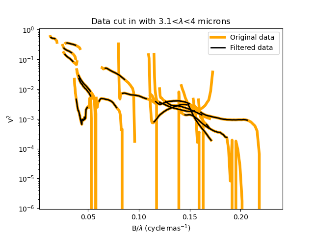
We first need to create a filter using one of the above function. For instance,
here we a simple filter to remove the edge of our MATISSE data with
the oimWavelengthRangeFilter.
class.
filt_wl = oim.oimWavelengthRangeFilter(wlRange=[3.1e-6, 4e-6])
The oimWavelengthRangeFilter
has two keywords:
targets: Which is common to all filter components: It specifies the targeted files within the data structure to which the filter applies. Possible values are: -"all"for all files (which we use in this example). - A single file specify by its index. - Or a list of indexes.wlRange: The wavelength range to cut as a two elements list (min wavelength and max wavelength), or a list of multiple two-elements lists if you want to cut multiple wavelengths ranges simultaneously. In our example you have selected wavelength between 3 and 4 microns. Wavelengths outside this range will be removed from the data.
We then apply the filter using th oimData.setFilter method
data.setFilter(filt_wl)
After applying a filter on an oimData instance,
this object will contain both the filtered and unfiltered data as two private members:
oimData._data: the unfiltered dataoimData._filteredData: the filtered data
oimData.datawill be point toward the filtereddata unless the member
oimData.data <oimodeler.oimData.oimData>.data()
We can temporary remove the filter by setting the
oimData.useFilter member to False
data.useFilter = False
or we can remove the filter once and for all using the the
oimData.setFilter method without argument.
data.setFilter()
Finally let’s plot the square visibility as the function of the spatial frequency for :
the unfiltered data in light grey.
the filtered data with a colorscale based on the wavlelength (in μm)
- To plot the unfiltered data without removing the filter we can use the
removeFilter=True option of the
oimData.plotmethod.
figcut,axcut = data.plot("SPAFREQ","VIS2DATA",yscale="log",xunit="cycle/mas",removeFilter=True,
                          label="Original data",color="orange",lw=4)
data.plot("SPAFREQ","VIS2DATA",axe=axcut,xunit="cycle/mas",label="Filtered data",color="k",lw=2)
axcut.legend()
axcut.set_title("Data cut in with 3.1<$\lambda$<4 microns")
A Few examples of filters
Spectral binning
Spectral binning can be applied easily using the
oimWavelengthBinningFilter
class. This might be useful to enhance the SNR on some noisy data or to reduce the
number data points in order to gain computing-time for model fitting.
- Here we are binning some HIGH resolution YSO data from GRAVITY by a factor 100
and plotting the raw and binned data.
dir0 = Path(__file__).resolve().parents[2] / "data" / "RealData" / "GRAVITY" / "HD58647"
filenames = list(dir0.glob("*.fits"))
data = oim.oimData(filenames)

filt_bin=oim.oimWavelengthBinningFilter(bin=100,normalizeError=False)
data.setFilter(filt_bin)

figbin,axbin = data.plot("SPAFREQ","VIS2DATA",yscale="log",xunit="cycle/mas",removeFilter=True,
                         label="Original data",color="orange",lw=4)
data.plot("SPAFREQ","VIS2DATA",axe=axbin,xunit="cycle/mas",label="Filtered data",color="k",lw=2)
axbin.legend()
axbin.set_title("Data binned by a factor of 100")

Flagging with expressions
- The
oimFlagWithExpressionFilter class can be used to remove data based on an expression based on standard OIFITS2 keywords (e.g. VIS2DATA, VIS2ERR, EFF_WAVE, UCOORD, MJD …) and a few additionnal quantities computed by oimodeler such as the baseline length (LENGTH) or orientation (PA).
Note
In the OIFITS2 format, all data extensions (OI_VIS2, OI_VIS, OI_T3, and OI_FLUX) contain a boolean column FLAG used to flag bad data. The flagged data are not used in oimodeler when computing \(chi^2\).
Typical use of the class
oimFlagWithExpressionFilter are :
flagging baselines based on length or orientation to perform specific model-fitting
flagging data based on relative errors
- For instance in the following we flag data with baselines longer than 50m for the MATISSE.
This can be useful to determine the caracterist size of object using simple models such as Gaussian or uniform disk and avoid being biased by longer baselines than would contain information on smaller structures.
path = Path(__file__).parent.parent.parent
dir0 = path / "data"  / "RealData" / "MATISSE"/ "FSCMa"
filenames = list(data_dir.glob("*.fits"))
data = oim.oimData(filenames)

filt_length=oim.oimFlagWithExpressionFilter(expr="LENGTH>50")
data.setFilter(filt_length)

figflag,axflag = data.plot("SPAFREQ","VIS2DATA",xunit="cycle/mas",removeFilter=True,
                            color="orange",label="Original data",lw=5)
data.plot("SPAFREQ","VIS2DATA",axe=axflag,xunit="cycle/mas",label="Filtered data",color="k",lw=2)
axflag.legend()
axflag.set_title("Removing (=flaggging) data where  B>50m")

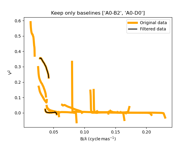
Selection by baseline name(s)
The oimKeepBaselinesFilter
class can be used to select data by baseline name. For instance in the following we
keep the data for the MATISSE data for the A0-B2 and A0-D0 baselines. Other data are
flagged and ths will not be used for chi2 computation and model fitting.
This can be useful to determine the caracterist size of object using simple models such as Gaussian or uniform disk and avoid being biased by longer baselines than would contain information on smaller structures.
path = Path(__file__).parent.parent.parent
dir0 = path / "data"  / "RealData" / "MATISSE"/ "FSCMa"
filenames = list(dir0.glob("*.fits"))
data = oim.oimData(filenames)

baselines=["A0-B2","A0-D0"]
filt_baselines=oim.oimKeepBaselinesFilter(baselines=baselines,arr="OI_VIS2")
data.setFilter(filt_baselines)
figflag,axflag = data.plot("SPAFREQ","VIS2DATA",xunit="cycle/mas",removeFilter=True,
                           color="orange",label="Original data",lw=5)
data.plot("SPAFREQ","VIS2DATA",axe=axflag,xunit="cycle/mas",
          label="Filtered data",color="k",lw=2)
axflag.legend()
axflag.set_title(f"Keep only baselines {baselines}")
Photometric and spectroscopic data
This complete code corresponding to this section is available in PhotometricAndSpectroscopicData.py
The OIFITS2 format
allow to use flux or spectrum measurements using the OI_FLUX extension.
The oimFluxdata class allows to convert flux
or spectroscopic measurement into and OIFITS file containing the OI_FLUX and extension as
well as the compulsory OI_WAVELENGTH, OI_TARGET and OI_ARRAY extensions.
To build some flux data you need to provide the oimFluxdata with:
oitarget: a OI_TARGET extension with the proper target name (can be copied from a OIFITS file)wl: the spectral channel central wavelengths for your flux/spectrum (unit in meter).dwl: the spectral channels width (can be put to some dummy values)flx: the fluxes measurements.flxerr: the uncertainties on the fluxes measurements.
Let’s assume that we have a 3 columns ascii files (named iso_spectrum_fname) for a ISO spectrum with: - the wavelengths in microns - the flux in Jansky, - and the uncertainties on the fluxes in Jansky.
The following code allows to load the ascii file, using
astropy.io.ascii
module, create a oimFluxdata object
and add it to some previously created oimData
object
isodata=ascii.read(iso_spectrum_fname)

wl  = isodata.columns['col1'].data*1e-6 # in m
dwl = 1e-9 #dwl is currently not used in oimodeler

flx = isodata.columns['col2'].data      # in Jy
err_flx = isodata.columns['col3'].data  # in Jy

oitarget=data.data[0]["OI_TARGET"].copy()

isoFluxData = oim.oimFluxData(oitarget,wl,dwl,flx,err_flx)
data.addData(isoFluxData)
The data can then used as standard OIFITS2 format data in oimodeler
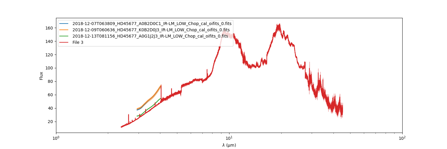
We can print the content of the data showing our ISO fluxes added as the third unamed file.
data.info()
════════════════════════════════════════════════════════════════════════════════
file 0: 2018-12-07T063809_HD45677_A0B2D0C1_IR-LM_LOW_Chop_cal_oifits_0.fits
────────────────────────────────────────────────────────────────────────────────
4)   OI_VIS2 :       (nB,nλ) = (6, 64)       dataTypes = ['VIS2DATA']
5)   OI_T3   :       (nB,nλ) = (4, 64)       dataTypes = ['T3PHI']
6)   OI_VIS  :       (nB,nλ) = (6, 64)       dataTypes = ['VISAMP', 'VISPHI']
7)   OI_FLUX :       (nB,nλ) = (1, 64)       dataTypes = ['FLUXDATA']
════════════════════════════════════════════════════════════════════════════════
file 1: 2018-12-09T060636_HD45677_K0B2D0J3_IR-LM_LOW_Chop_cal_oifits_0.fits
────────────────────────────────────────────────────────────────────────────────
4)   OI_VIS2 :       (nB,nλ) = (6, 64)       dataTypes = ['VIS2DATA']
5)   OI_T3   :       (nB,nλ) = (4, 64)       dataTypes = ['T3PHI']
6)   OI_VIS  :       (nB,nλ) = (6, 64)       dataTypes = ['VISAMP', 'VISPHI']
7)   OI_FLUX :       (nB,nλ) = (1, 64)       dataTypes = ['FLUXDATA']
════════════════════════════════════════════════════════════════════════════════
file 2: 2018-12-13T081156_HD45677_A0G1J2J3_IR-LM_LOW_Chop_cal_oifits_0.fits
────────────────────────────────────────────────────────────────────────────────
4)   OI_VIS2 :       (nB,nλ) = (6, 64)       dataTypes = ['VIS2DATA']
5)   OI_T3   :       (nB,nλ) = (4, 64)       dataTypes = ['T3PHI']
6)   OI_VIS  :       (nB,nλ) = (6, 64)       dataTypes = ['VISAMP', 'VISPHI']
7)   OI_FLUX :       (nB,nλ) = (1, 64)       dataTypes = ['FLUXDATA']
════════════════════════════════════════════════════════════════════════════════
file 3:
────────────────────────────────────────────────────────────────────────────────
4)   OI_FLUX :       (nB,nλ) = (1, 29510)    dataTypes = ['FLUXDATA']
════════════════════════════════════════════════════════════════════════════════
We can plot the spectrum of the MATISSE and ISO data to compare them (note that they are both in Jansky).
data.plot("EFF_WAVE","FLUXDATA",color="byFile",xunit="micron",errorbar=True)