Model fitting

In the oimodeler framework, model-fitting is performed by classes deriving from the abstract class oimFitter. Here we describe the common functionalities and methods of these fitting classes.

Theses classes encapsulate an oimSimulator instance, which determines the \(\chi^2\) value between the data and the model as seen in the Data/Model comparison section. As for the simulator class, \(\chi^2\) can be computed only on a subset of datatypes setting the dataTypes kewyord.

When creating a oimFitter the user should either pass an instance of oimSimulator

fit = oimFitter(sim)

or an instance of oimData and oimModel

fit = oimFitter(data, model)

The fitting classes have four common methods:

• prepare : prepare the fitter: defining the parameter space…

• run : launch the model-fitting run

• getResults : return the best-fit parameters and uncertainties

• printResults : print the result of the model-fitting

Warning

After calling the getResults or printResults the parameters of the oimModel is set to their best-fit values.

The various classes of model-fitting also includes specific plotting functions that will be described in details in their recpective sub-sections.

In the current version, oimodeler includes four model-fitting algorithms.

Available Model-Fitters

Fitter Name	Description
oimFitter	Abstract class for model-fitting
oimFitterEmcee	MCMC sampler (based on the emcee python package)
oimFitterDynesty	Dynamic/static nested sampler (based on the the dynesty package)
oimFitterMinimize	a simple \(\chi^2\) minimizer using the numpy Minimize function
oimFitterRegularGrid	regular grid with \(\chi^2\) explorer

These various algorithms allow the user to find the best-fit values of all free parameters of the model (minimum of \(\chi^2\)) and, depending on their nature, to evaluate their statistic.

For instance, uncertainties can be estimated using :

• the posterior probability function in the case of MCMC or DNS

• the covariant matrix for the gradient-descent methods such as Minimize one

Warning

It should be noted that no model fitting algorithm can guarantee convergence to the global minimum of the chi-squared statistic.

Emcee fitter

A few words about the MCMC algorithm

The Markov Chain Monte Carlo (MCMC) algorithm is a method used to sample from complex probability distributions when direct sampling is difficult. It works by constructing a Markov chain, a sequence of random variables where each variable depends only on the previous one.

Unlike optimization algorithms that seek the global minimum, MCMC methods do not directly aim to find it. Instead, they converge toward a probability distribution, which may be concentrated near the global minimum if that region has high probability.

The burn-in phase refers to the initial iterations of the MCMC process, during which the chain has not yet reached the target distribution and the samples may not be representative of the true posterior.

After a burning phase, the chain “wanders” over time through the sample space in such a way that the frequency of visits to each region reflects the target distribution, allowing for approximate estimation of expectations and probabilities.

Description of the oimFitterEmcee class

To implement a MCMC sampler, oimodeler use the python library emcee. If you are not confident with this package, you should have a look at the documentation here.

The emcee sampler is encapsulated into the oimFitterEmcee class.

At the creation of the fitter the number of desired walker exploring the paramter space can be specified using the keyword nwalkers. The default number is 20.

fit = oim.oimFitterEmcee(data,model, nwalkers=10, dataTypes=["VIS2DATA","T3PHI"])

The prepare method should then be called to set the initial walkers positions. Two options are available depending on the value of the keyword init:

• random : (default) Uniformly random positions within the parameter space limited by the values of oimParam.min and oimParam.max

• gaussian : random positions from a normal (Gaussian) distribution around the current position defined by the oimParam.value with standard deviation of oimParam.error

The oimFitterEmcee class offers two additionnal functionalities of the emcee package.

The first one is the possiblity of changing the walker moves to optimize the parameter space exploration.

The user can also load and save the sampler using the HDF5 backend. This can be done by specifying an hdf5 file with the samplerFile keyword. If the file exists, it is loaded into the sampler. Its probability distribution can be explored and the best-fit parameters determined. If the file doesn’t exist, it will be created and the results of the MCMC run will be saved in this file.

fit.prepare(init="gaussian", moves = moves.StretchMove, samplerFile=mySampler.h5)

After initializing the walkers, the MCMC run can be performed using the run method. The number of iterations of the run is set by the nsteps keyword. The progress keyword can be used to show a progress bar.

fit.run(nsteps=5000, progress=True)

After the MCMC run, the results can be plotted with three methods:

Example on MIRCX data of a binary star

To demonstrate the use of the oimFitterEmcee class we will use a single MIRCX observation of the binary star \(\beta\) Ari. The code for this section is in emceeFitting.py

We start by creating a binary star model conissting of two uniform disk components.

ud1 = oim.oimUD()
ud2 = oim.oimUD()
model = oim.oimModel([ud1, ud2])

Before starting the run, we need to specify which parameters are free and what their ranges are. By default, all parameters are free, but the components x and y coordinates. For a binary, we need to release them for one of the components. As we only deal with relative fluxes, we can normalize the total flux to one.

ud1.params["d"].set(min=0, max=2)
ud1.params["f"].set(min=0.8, max=1)
ud2.params["d"].set(min=0, max=2)
ud2.params["x"].set(min=-100, max=100, free=True)
ud2.params["y"].set(min=-100, max=100, free=True)
model.normalizeFlux()

We can print the list of free paramaters of our binary model:

model.getFreeParameters()

{'c1_UD_d': oimParam at 0x2031db6e7e0 : d=0 ± 0 mas range=[0,2] free=True ,
'c1_UD_f': oimParam at 0x2031ee86db0 : f=1 ± 0  range=[0.8,1] free=True ,
'c2_UD_d': oimParam at 0x2031f530d40 : d=0 ± 0 mas range=[0,2] free=True ,
'c2_UD_x': oimParam at 0x2031bf4ae40 : x=0 ± 0 mas range=[-100,100] free=True ,
'c2_UD_y': oimParam at 0x2031f4bf1d0 : y=0 ± 0 mas range=[-100,100] free=True }

We load the MIRCX data and filter out the OI_VIS table to reduce computation time.

data=oim.oimData(file)
filt=oim.oimRemoveArrayFilter(arr="OI_VIS")
data.setFilter(filt)

We then create the emcee fitter. We set of number of walkers to 12 and specify that theonly the VIS2DATA and T3PHI we will be used to compute the \(\chi^2\).

Note

emcee requires the number of walkers to be at least twice the number of free parameters.

We need to initialize the fitter using its oimFitterEmcee.prepare method. This method is setting the initial values of the walkers either in Gaussian or uniform distribution (see previous section). The default method is to set them to random values within the parameters range.

fit.prepare()

The variable initialParams of the oimFitterEmcee instance contains the initial values the parmaters for all walkers.

print(fit.initialParams)

array([[ 8.95841039e-01,  6.60835250e-01,  5.97499196e+01,
     7.54750698e+01,  1.34828828e+00],
   [ 9.90477053e-01,  1.18066929e+00,  7.42332565e+01,
    -7.74195309e+01,  1.01373315e+00],
   [ 8.61175261e-01,  9.73948406e-03,  8.41031622e+01,
     9.65519546e+01,  1.98837369e+00],
   [ 8.74741367e-01,  1.83656376e+00, -2.13259171e+01,
    -8.35083861e+01,  1.61472161e+00],
   [ 9.45848256e-01,  6.95701956e-01,  9.52905809e+01,
     4.21371881e+01,  8.68078468e-01],
   [ 8.15209564e-01,  6.63088192e-01,  3.81774226e+01,
    -5.21909577e+01,  1.63010167e+00],
   [ 8.62539242e-01,  1.41065537e+00,  7.72304319e+01,
    -3.98899413e+01,  1.91458275e+00],
   [ 9.20929111e-01,  1.90288993e-02, -5.30189260e+01,
     5.06516249e+01,  7.38609144e-01],
   [ 9.72689492e-01,  6.04406879e-01,  3.26247393e+01,
     6.20385451e+01,  2.59662765e-01],
   [ 8.32000110e-01,  7.87671717e-01, -7.31812757e+01,
     1.76352972e+01,  1.81975894e+00],
   [ 9.89702924e-01,  8.08596701e-01, -7.59071858e+01,
     8.88992214e+01,  1.13866453e-01],
   [ 9.24424779e-01,  9.79528699e-01,  7.12641054e+01,
     4.48065035e+00,  1.93515687e+00]])

We can now run the fit. We choose to run 20000 steps as a start and interactively show the progress with a progress bar. The fit should take a few minutes on a standard computer to compute around 240000 models (nwalkers x nsteps).

fit.run(nsteps=20000, progress=True)

The oimFitterEmcee instance stores the emcee sampler as an attribute: oimFitterEmcee.sampler. You can, for example, access the chain of walkers and the logrithmic of the probability directly.

sampler = fit.sampler
chain   = fit.sampler.chain
lnprob  = fit.sampler.lnprobability

We can directly manipulate or plot these data. However, the oimFitterEmcee implements various methods to retrieve and plot the results of the mcmc run.

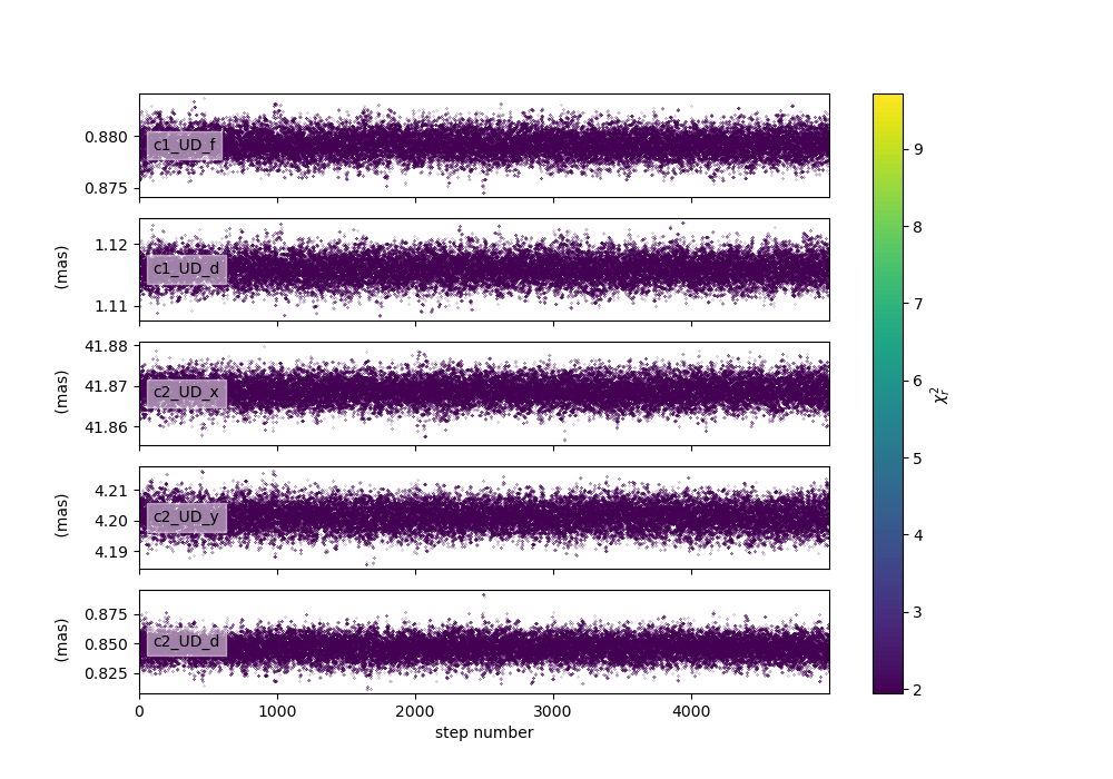
The walkers position as the function of the steps with a \(\chi^2\) color scale can be plotted using the oimFitterEmcee.walkersPlot method. This method have the following parameters (default in parenthesis):

• savefig (None) : path of the file to save the plot

• chi2limfact (20) : define the upper limit of the color scale in \(\chi^2\)

• labelsize (10) : size of the label of the parameters name

• ncolors (128) : number of colors for the color scale (reduce if the function is too slow for large sample)

Let’s plot the evolution of the walkers with a limit of 10 tiimes the minimum \(\chi^2\).

figWalkers, axeWalkers = fit.walkersPlot(chi2limfact=10)

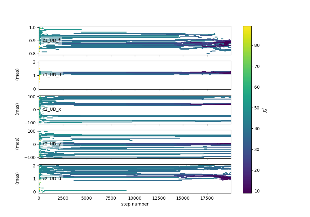
As evidenced in this figure 20000 steps is not enough for the MCMC run to converge aroun the globaml minimum of \(\chi^2\) : - not all walkers are around the same positions - the \(\chi^2\) is still quite high (but this could also be due to a choice of bad model) - the positions are not yet stable as a function of time

Let’s add 20000 steps by running again the same fitter.

Note

By default the oimFitterEmcee.run method starts at the current position of the walker. The option reset can be specified to reset the sampler to the initial positions.

fit.run(nsteps=20000, progress=True)

Let’s plot the walkers positions for the 40000 steps.

figWalkers2, axeWalkers2 = fit.walkersPlot(chi2limfact=10)

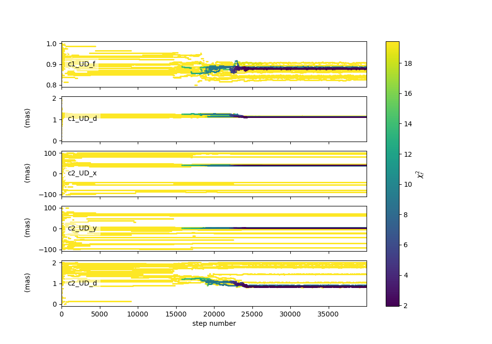
Although not all walkers have converged to the same position, a group of them has converged to a location yielding a significantly lower \(\chi^2\). Moreover, the positions of most walkers appear to have remained stable for at least 10,000 steps.

Although there is no mathematical test to determine whether the position corresponds to the global minimum of the \(\chi^2\), we will assume that the walkers clustered around this minimum have converged to the global minimum, while the others are trapped in local minima. As we will see using the grid fitter, this behavior often occurs with binary data.

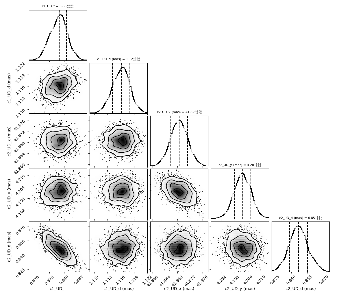
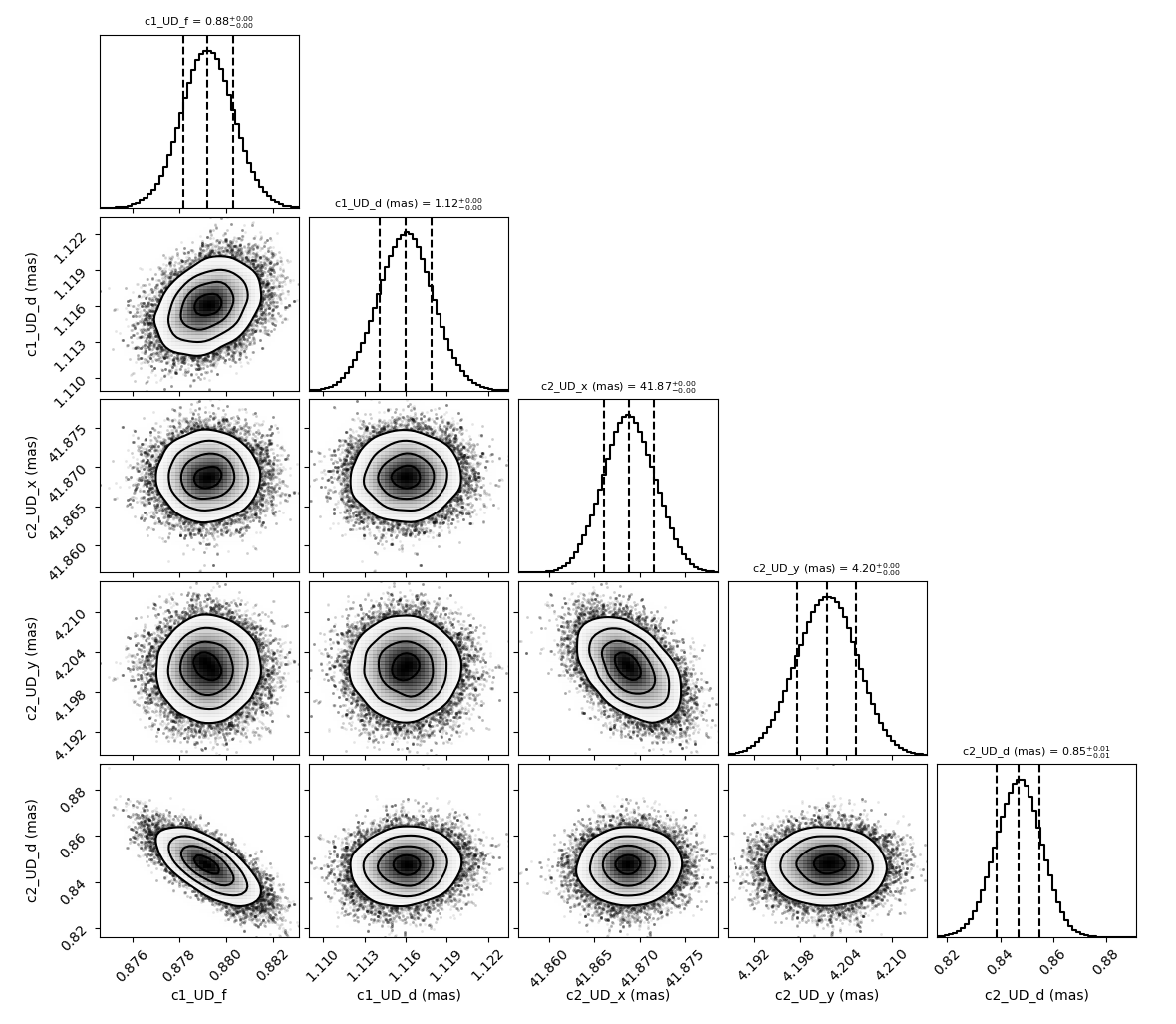
We can generate the well-known corner plot, which displays both 1D and 2D density distributions of the parameters. The oimodeler package uses the corner library for this purpose. To ensure we are analyzing only the converged part of the chains, we discard the first 35,000 steps, as most walkers have converged after that point.

By default, the corner plot also excludes samples with a :math:chi^2 value more than 20 times higher than that

of the best-fit model. This cutoff can be adjusted using the chi2limfact keyword of the

oimFitter.cornerPlot method.

However, since not all walkers have converged to the global minimum, we will use a lower value for this parameter to ensure that only the walkers clustered around the global minimum are included in the posterior distribution.

figCorner, axeCorner=fit.cornerPlot(discard=35000, chi2limfact=3)

We can now retrieve the results of the fit. The oimFitterEmcee function can return the best, mean, or median model, depending on the selected option. It also provides uncertainties estimated from the posterior density distribution

(see the emcee documentation for more details).

median, err_l, err_u, err = fit.getResults(mode='median', discard=35000, chi2limfact=3)

To compute the median and mean models, we must first exclude, as in the corner plot, the walkers that did not converge. This is done using the chi2limfact keyword (default is again 20). We also remove the burn-in phase using the discard option.

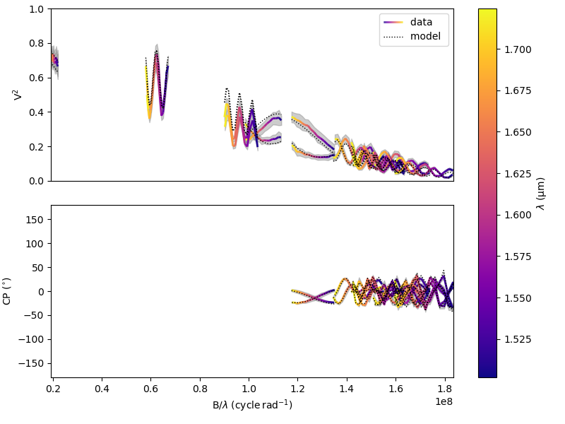
When retrieving the results, the simulated data is automatically generated using the fitter’s internal simulator. We can then plot the data and model again, and compute the final reduced chi-squared \(\chi^2_r\):

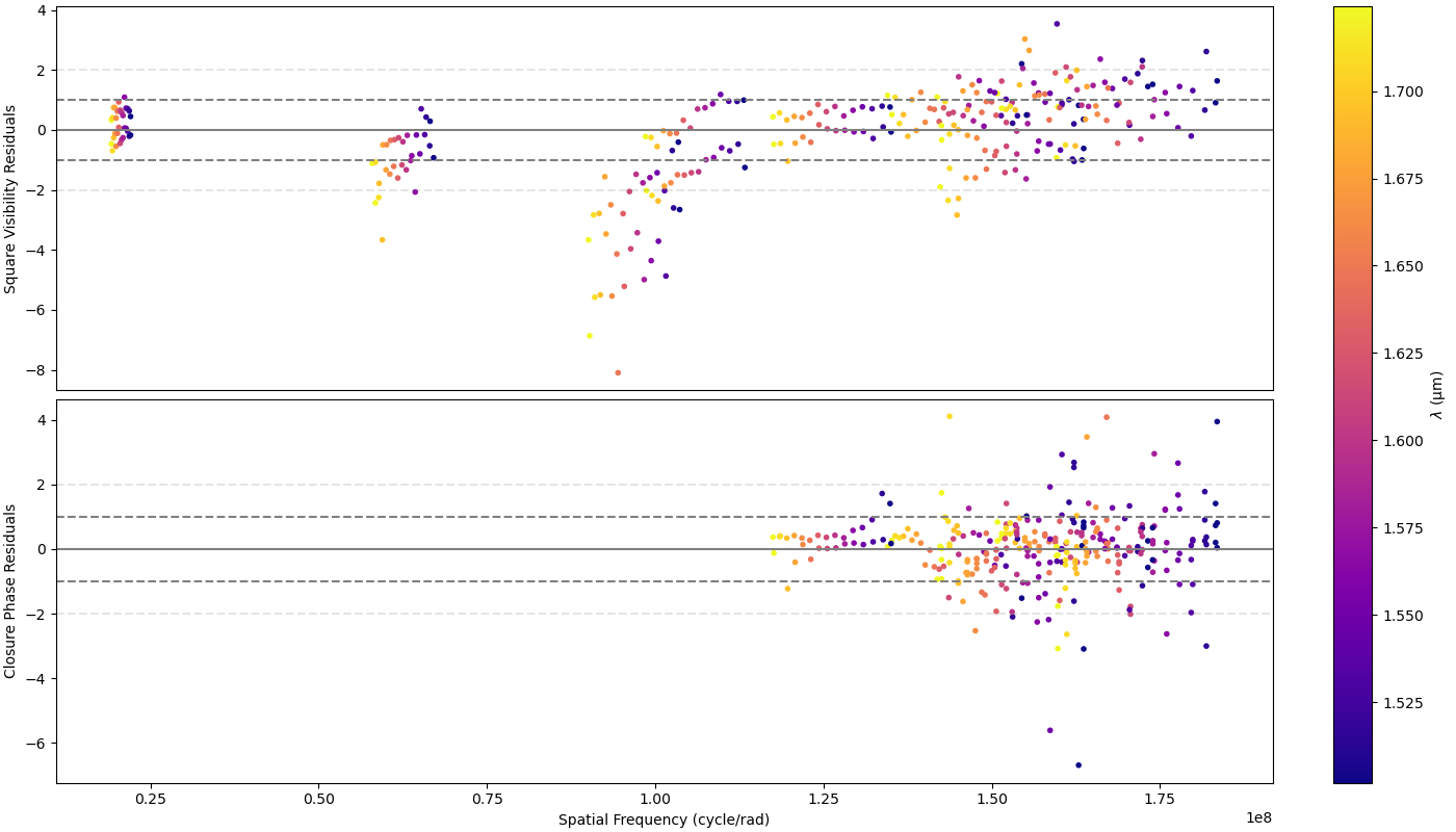
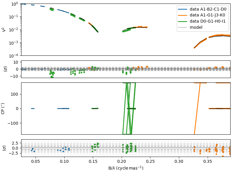
figSim, axSim=fit.simulator.plot(["VIS2DATA", "T3PHI"])
pprint("Chi2r = {}".format(fit.simulator.chi2r))

We can also plot the fit residuals using the plotResiduals of the oimSimulator class.

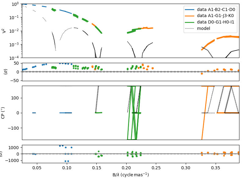
fig2, ax2 = fit.simulator.plotResiduals(["VIS2DATA", "T3PHI"],levels=[1,2])

We note that using a low value for the chi2limfact option is effective in removing walkers that have not converged but biases the posterior distribution.

To obtain a more robust estimate, we can create a new oimFitterEmcee instance, initialize the parameters using a Gaussian distribution around the putative global minimum (using the currently estimated uncertainties on the parameters as the Gaussian sigma), and run it for several thousand steps.

To ensure that the initialization is properly performed, we first use the oimFitterEmcee.getResults method, which sets the model parameters and uncertainties according to the results from the first fitter.

fit.getResults(mode="best", discard=35000, chi2limfact=3)
fit2 = oim.oimFitterEmcee(data, model, nwalkers=20,dataTypes=["VIS2DATA","T3PHI"])
fit2.prepare(init="gaussian")
fit2.run(nsteps=5000, progress=True)

We can then display the walker and corner plots.

figWalkers, axeWalkers = fit2.walkersPlot(chi2limfact=5)
figCorner, axeCorner = fit2.cornerPlot(discard=2000)

We can also print the reuslts:

fit2.printResults(mode="best", discard=2000)

c1_UD_f = 0.87928 ± 0.00106
c1_UD_d = 1.11597 ± 0.00191 mas
c2_UD_x = 41.86875 ± 0.00276 mas
c2_UD_y = 4.20204 ± 0.00383 mas
c2_UD_d = 0.84589 ± 0.00811 mas
chi2r = 1.95965

And, finally, we can then plot the data and model comparison and the residual simultaneously using the plotWithResiduals of the oimSimulator class.

fig2, ax2 = fit2.simulator.plotWithResiduals(["VIS2DATA", "T3PHI"],levels=[1,2,3],
                     xunit="cycle/mas",kwargsData=dict(color="byBaseline",marker="."))

\(\chi^2_r\) Minimizer

oimodeler also implements oimFitterMinimize, a simple \(\chi^2_r\) minimization fitter based on the minimize function provided by the scipy Python package.

To demonstrate it’s use o we will use three VLTI/PIONIER observations of the supergiant Canopus taken from Domiciano de Souza et al. 2021 paper. The code for this section is in simpleMinimizerFitting.py .

First, we load the data into an instance of oimData.

data_dir = path / "data" / "RealData" "/PIONIER" / "canopus"
files = list(data_dir.glob("PION*.fits"))
data=oim.oimData(files)

We create a model, here a single component of a powerlaw limb-darkened disk.

pldd = oim.oimPowerLawLDD(d=8, a=0)
model = oim.oimModel(pldd)
model.normalizeFlux()

We create an instance of the oimFitterMinimize class, prepare the fitter, run it, and finally print the results.

lmfit = oim.oimFitterMinimize(data, model,dataTypes=["VIS2DATA", "T3PHI"])
lmfit.prepare()
lmfit.run()
lmfit.printResults()

c1_PLLDD_d = 7.24385 ± 0.00472 mas
c1_PLLDD_a = 0.19947 ± 0.00310
chi2r = 6.06760

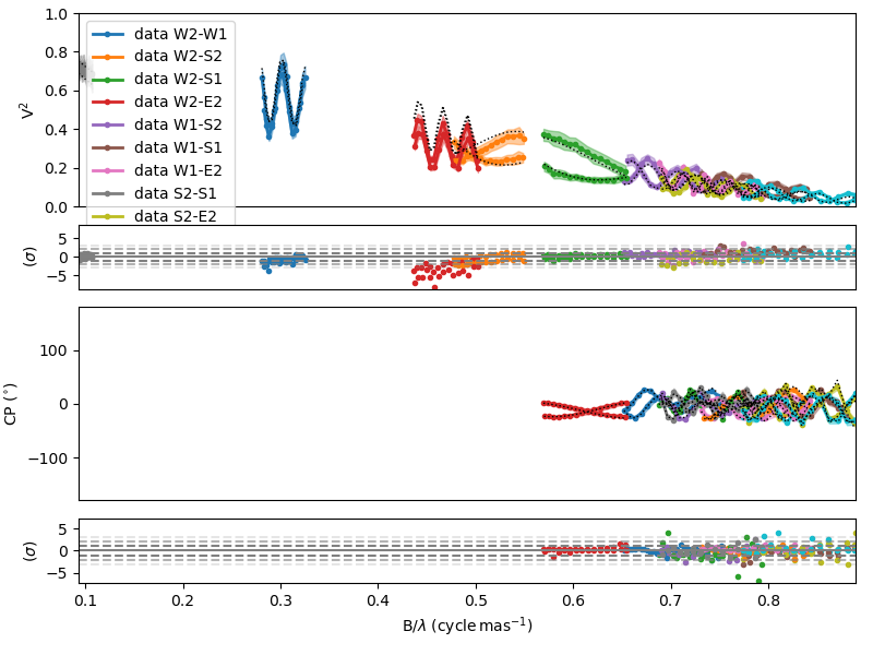
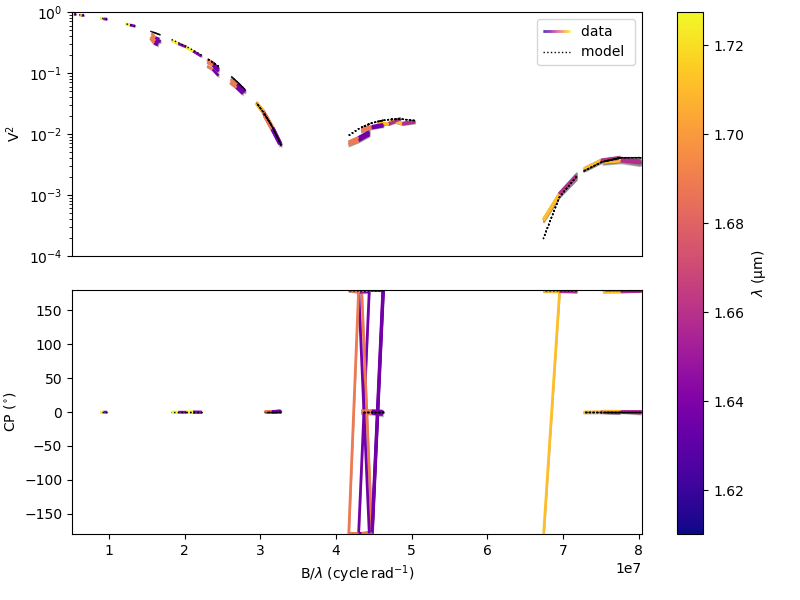
Finally, we can plot the comparison obetween our PIONIER data and our model and the residual.

fig, ax = lmfit.simulator.plotWithResiduals(["VIS2DATA", "T3PHI"],xunit="cycle/mas",
                                          kwargsData=dict(color="byConfiguration"))

ax[0].set_yscale("log")
ax[0].set_ylim(1e-4,1)

Warning

The minimize fitter only converge to the closest local minimum.

For instance, let’s see what happens when we start with an initial diameter of 15 mas. We can modify the

pldd.params["d"].value=10
lmfit.prepare()
lmfit.run()
lmfit.printResults()

c1_PLLDD_d = 14.78362 ± 1.43824 mas
c1_PLLDD_a = 0.06933 ± 0.30199
chi2r = 35948.20365

The minimizer converge to a local minimum with a high value of the \(\chi^2_r\).

We can plot the data-to-model comparison to verify that the fit is poor.

fig2, ax2 = lmfit.simulator.plotWithResiduals(["VIS2DATA", "T3PHI"],xunit="cycle/mas",
                                          kwargsData=dict(color="byConfiguration"))

ax2[0].set_yscale("log")
ax2[0].set_ylim(1e-4,1)

Note that the minimization method can be specified using the method keyword during instantiation. The list of available methods, along with their pros and cons, is described in

the SciPy minimize documentation .

For instance to use the Broyden–Fletcher–Goldfarb–Shanno (BFGS) algorithm:

lmfit2 = oim.oimFitterMinimize(data, model,
                  dataTypes=["VIS2DATA", "T3PHI"], method="BFGS")

Note

One of the main advantages of the minimizer fitter is that it provides an alternative estimation of the uncertainties on the free parameters, i.e., based on the covariance matrix, compared to the MCMC method, which relies on the statistics of the posterior probability function.

Regular Grid exploration

oimodeler implements, oimFitterGrid, a simple tool to create grids of \(\chi^2_r\) as a function of parameters values.

Here, we explain how to use this fitter to explore the parameter space of omdels of the stellar surface of the giant star Canopus observed by VLTI/PIONIER instrument.

The code is available on the oimodeler github: gridFitting.py .

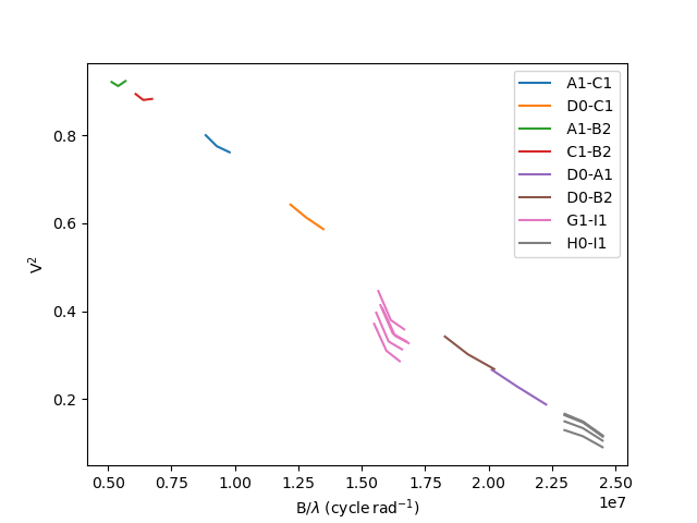
Let’s first load the data and plot the uu plan and the square visibility:

data = oim.oimData(fdata)

fig,ax = plt.subplots(1,2,subplot_kw=dict(projection='oimAxes'),
                     figsize=(15,6))
data.uvplot(color="byBaseline",axe=ax[0])
data.plot("SPAFREQ","VIS2DATA",color="byBaseline",
         axe=ax[1],xunit="cycle/mas",errorbar=True)
ax[1].set_yscale("log")

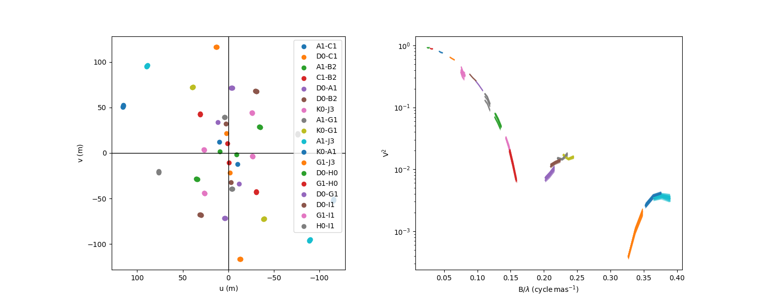
The visibility plot show that Canopus is over-resolved by most of the baselines and we clearly see the second and third lobe of the visibility so that we should be able to constrain the limb-darkening.

But first, we’ll fit the data using a uniform disk model. Let’s build this model

ud = oim.oimUD()
mud = oim.oimModel(ud)
mud.normalizeFlux()

We will use oimFitterGrid fitter to explore the unique parameter of this model: the uniform disk diameter.

First, as for all oimodeler fitters, we create the instance and give it some data and some model. We can specify which data types should be included in the \(\chi^2_r\) computation using the dataTypes option. Here we chose to include both the square visibility and closure phase.

grid = oim.oimFitterRegularGrid(data,mud,dataTypes=["VIS2DATA","T3PHI"])

We then prepare the grid by specifying :

• the parameter(s) to explore using the params options.

• range to explore for each parameter using the min and max options.

• the steps size for each parameter, here 0.05 mas.

Finally, we can run the grid:

grid.run()

This one-dimensional grid is fast to compute, as there are only 62 models for which the \(\chi^2_r\) needs to be evaluated.

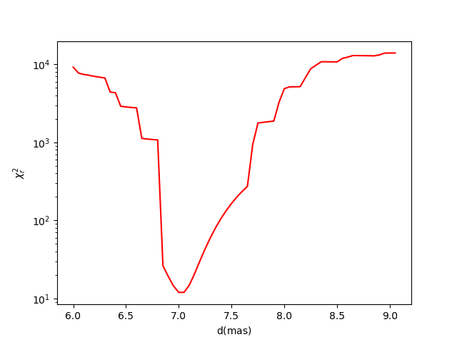
We can now plot the result using the oimFitterGrid.plotMap method.

fig_grid, ax_grid = grid.plotMap()
ax_grid.set_yscale("log")

The “best-fit” from the grid exploration can be returned using the oimFitter.getResults oimFitter.getResults or oimFitter.plotResults mehtods.

grid.printResults()

d = 7.00000 mas
chi2r = 11.97244

Note

Unlike other fitters, no uncertainties are computed from the grid exploration, and the best-fit parameters obtained do not correspond to a true \(\chi^2_r\) minimum, but are limited by the step size.

In order to go beyond this limit one can combined the oimFitterGrid with a oimFitterMinimize fitter.

Our starting point for the \(\chi^2_r\) minimizer is the best-fit parameter from the grid.

miniz = oim.oimFitterMinimize(data,mud,dataTypes=["VIS2DATA","T3PHI"])
miniz.prepare()
miniz.run()
miniz.printResults()

c1_UD_d = 7.02461 ± 0.00118 mas
chi2r = 11.65689

We can now plot the fitted data using the oimSimulator.plot method

fig_sim, ax_sim = grid.simulator.plot(["VIS2DATA","T3PHI"])
ax_sim[0].set_yscale("log")
ax_sim[0].set_ylim(1e-4,1)

Let’s now perform a 2D grid exploration using the power-law limb darkened model.

pld = oim.oimPowerLawLDD()
mpldd=oim.oimModel(pld)
mpldd.normalizeFlux()

grid2 = oim.oimFitterRegularGrid(data,mpldd,dataTypes=["VIS2DATA","T3PHI"])
grid2.prepare(params=[pld.params["d"],pld.params["a"]],min=[6,0],max=[9,2],steps=[0.05,0.05])
grid2.run()

Here we explore the limb-darkened diameter d and the limb-darkened power a.

We then plot the resulting 2D map of the \(\chi^2_r\).

fig2_grid2, ax_grid2 = grid2.plotMap(plotContour=True,
                                    contour_kwargs=dict(levels=[2,4]),
                                    norm=colors.LogNorm(),cmap="plasma")

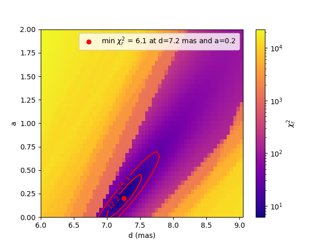
As seen in the example above the oimFitterGrid.plotMap method allows some plot customization: - plotContour allows to plot contours of \(\chi^2_r\) - contour_kwargs are keywords passed to the matplotlib contour function - norm allows the image colors normalization

Note

The levels are defined as multiples of the minimum \(\chi^2_r\). In this case, we have plotted the contours at 2 and 4 times the minimum \(\chi^2_r\).

Grid exploration isparticularly interesting to vizualize: - correlations or even degeneracy between parameters - the presence of multiple \(\chi^2_r\) local minima

In the plot above, we clearly see a correlation between the disk diameter d and the exponent a of the limb-darkening law. This correlation would become a degeneracy if we did not have measurements beyond the first zero of the visibility.

Let’s filter out the baselines longer than 40m using the oimFlagWithExpressionFilter filter.

filt_B = oim.oimFlagWithExpressionFilter(expr="LENGTH>40")
data.setFilter(filt_B)

We plot the VIS2DATA to verify that we do not reach the first zero of the visibility.

fig,ax = data.plot(“SPAFREQ”,”VIS2DATA”,color=”byBaseline”) ax.legend()

Finally, we create a new 2D grid fitter with the same parameters as before and plot the resulting \(\chi^2_r\) map.

grid3 = oim.oimFitterRegularGrid(data,mpldd,dataTypes=["VIS2DATA","T3PHI"])
grid3.prepare(params=[pld.params["d"],pld.params["a"]],
              min=[6,0],max=[9,2],steps=[0.05,0.05])
grid3.run()

fig_grid3, ax_grid3 = grid3.plotMap(plotContour=True,
                                    contour_kwargs=dict(levels=[2,4]),
                                    norm=colors.LogNorm(),cmap="plasma")

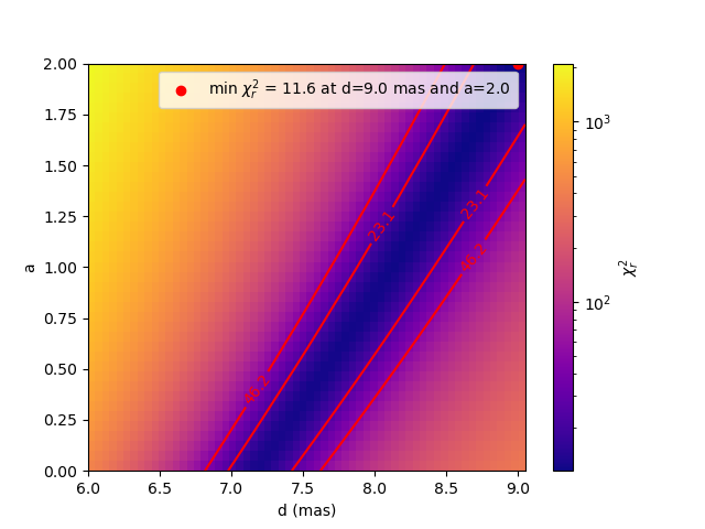
Now, we clearly see the degeneracy between the disk diameter d and the exponent a of the limb-darkening law, which highlights the need to obtain measurements beyond the first zero of visibility to better constrain the limb-darkening of stars.

Let’s finish this section by having a look at some binary data.

Dynesty fitter

The oimodeler package also implements oimFitterDynesty, a fitter based on the dynesty package. This fitter uses Dynamic Nested Sampling (DNS) to estimate Bayesian posteriors and model evidences.

Documentation on that fitter will be added later.

About uncertainties on parameters