Building and using models

The basics of models

This complete code corresponding to this section is available in TheBasicsOfModels.py

Models, Components and Parameters

In the oimodeler framework, a model is and instance of the oimModel class. It contains a collection of components, which all derived from the oimComponent semi-abstract class. The components may be described in the image plane, by their 1D or 2D intensity distribution, or directly in the Fourier plane, for the most simple components with known analytical Fourier transforms. Each components is described by a set of parameters which are instances of the oimParam class.

Thus, building models in oimodeler relies on three classes:

• oimModel: the model class

• oimComponent: the abstract class from which all components derive

• oimParam: the parameter class

To create models we must first create some components. Let’s create a few simple components.

pt = oim.oimPt(f=0.1)
ud = oim.oimUD(d=10, f=0.5)
g  = oim.oimGauss(fwhm=5, f=1)
r  = oim.oimIRing(d=5, f=0.5)

Here, we have create a point source, a 10 mas uniform disk, a Gaussian distribution with a 5 mas fwhm and a 5 mas infinitesimal ring. The comprehensive list of components available is oimodeler is given in the next section.

The model parameters which are not set explicitly during the components creation are set to their default values (i.e., f=1, x=y=0).

We can print the description of the component easily:

print(ud.params)

Uniform Disk x=0.00 y=0.00 f=0.50 d=10.00

Or if you want to print the details of a parameter:

print(ud.params['d'])

oimParam d = 10 ± 0 mas range=[-inf,inf] free

Note that the components parameters are instances of the oimParam class which hold not only the parameter value stored in the oimParam.value attribute, but in addition to it the following attributes:

• oimParam.error: the parameters uncertainties (for model fitting).

• oimParam.unit: the unit as a astropy.units object.

• oimParam.min: minimum possible value (for model fitting).

• oimParam.max: minimum possible value (for model fitting).

• oimParam.free: Describes a free parameter for True and a fixed parameter for False (for model fitting).

• oimParam.description: A string that describes the model parameter.

Building Models

We can now create our first models using the oimModel class.

mPt   = oim.oimModel(pt)
mUD   = oim.oimModel(ud)
mG    = oim.oimModel(g)
mR    = oim.oimModel(r)
mUDPt = oim.oimModel(ud, pt)

Now, we have four one-component models and one two-component model.

We can get the parameters of our models using the oimModel.getParameters method.

params = mUDPt.getParameters()
print(params)

{'c1_UD_x': oimParam at 0x23de5c62fa0 : x=0 ± 0 mas range=[-inf,inf] free=False ,
 'c1_UD_y': oimParam at 0x23de5c62580 : y=0 ± 0 mas range=[-inf,inf] free=False ,
 'c1_UD_f': oimParam at 0x23de5c62400 : f=0.5 ± 0  range=[-inf,inf] free=True ,
 'c1_UD_d': oimParam at 0x23debc1abb0 : d=10 ± 0 mas range=[-inf,inf] free=True ,
 'c2_Pt_x': oimParam at 0x23debc1a8b0 : x=0 ± 0 mas range=[-inf,inf] free=False ,
 'c2_Pt_y': oimParam at 0x23debc1ab80 : y=0 ± 0 mas range=[-inf,inf] free=False ,
 'c2_Pt_f': oimParam at 0x23debc1ac10 : f=0.1 ± 0  range=[-inf,inf] free=True }

The method returns a dict of all parameters of the model components. The keys are defined as

x{num of component}_{short Name of component}_{param name}.

Alternatively, we can get the free parameters using the getFreeParameters method:

freeParams = mUDPt.getParameters()
print(freeParams)

{'c1_UD_f': oimParam at 0x23de5c62400 : f=0.5 ± 0  range=[-inf,inf] free=True ,
 'c1_UD_d': oimParam at 0x23debc1abb0 : d=10 ± 0 mas range=[-inf,inf] free=True ,
 'c2_Pt_f': oimParam at 0x23debc1ac10 : f=0.1 ± 0  range=[-inf,inf] free=True }

The two main methods of an oimModel object are:

• getImage: which returns an image of the model

• oimModel.getComplexCoherentFlux which returns the complex Coherent Flux of the model

Althought the getImage is only used to vizualize the model intensity distribution and is not used for model-fitting, getComplexCoherentFlux is at the base of the computation of all interferometric observables and thus of the data-model comparison.

Getting the model image

Let’s first have a look at the oimModel.getImage method.

It takes two arguments, the image’s size in pixels and the pixel size in mas.

im = mUDPt.getImage(512, 0.1)
plt.figure()
plt.imshow(im**0.2)

We plot the image with a 0.2 power-law to make the uniform disk components visible: Both components have the same total flux but the uniform disk is spread on many more pixels.

The image can also be returned as an astropy hdu object (instead of a numpy array) setting the toFits keyword to True. The image will then contained a header with the proper fits image keywords (NAXIS, CDELT, CRVAL, etc.).

im = mUDPt.getImage(256, 0.1, toFits=True)
print(im)
print(im.header)
print(im.data.shape)

... <astropy.io.fits.hdu.image.PrimaryHDU object at 0x000002610B8C22E0>

SIMPLE  =                    T / conforms to FITS standard
BITPIX  =                  -64 / array data type
NAXIS   =                    2 / number of array dimensions
NAXIS1  =                  256
NAXIS2  =                  256
EXTEND  =                    T
CDELT1  = 4.84813681109536E-10
CDELT2  = 4.84813681109536E-10
CRVAL1  =                    0
CRVAL2  =                    0
CRPIX1  =                128.0
CRPIX2  =                128.0
CUNIT1  = 'rad     '
CUNIT2  = 'rad     '
CROTA1  =                    0
CROTA2  =                    0

(256, 256)

Note

Currently only regular grids in wavelength and time are allowed when exporting to fits-image format. If specified, the wl and t vectors need to be regularily sampled. The easiest way is to use the numpy.linspace function.

If their sampling is irregular an error will be raised.

Using the oimModel.saveImage method will also return an image in the fits format and save it to the specified fits file.

im = mUDPt.saveImage("modelImage.fits", 256, 0.1)

Note

The returned image in fits format will be 2D, if time and wavelength are not specified, or if they are numbers, 3D if one of them is an array, and 4D if both are arrays.

Alternatively, we can use the oimModel.showModel method which take the same argument as the getImage, but directly create a plot with proper axes and colorbar.

figImg, axImg = mUDPt.showModel(512, 0.1, normPow=0.2)

Getting the model Complex Coherent Flux

In most of the cases the user won’t use directly the oimModel.getComplexCoherentFlux method to retrieve the model complex coherent flux for a set of coordinates but will create oimSimulator or a oimSimulator that will contain the instance of oimModel and some interferometric data in an oimData to simulate interferometric quantities from the model at the spatial frequenciesfrom our data. This will be covered in the XXXXXXXXXXX section.

Nevertheless, in some cases and for explanatory purposes we will directly use this methods in the following example. Without the oimSimulator class, the oimModel can only produce complex coherent flux (i.e., non normalized complex visibility) for a vector of spatial frequecies and wavelengths.

wl = 2.1e-6
B = np.linspace(0.0, 300, num=200)
spf = B/wl

Here, we have created a vector of 200 spatial frequencies, for baselines ranging from 0 to 300 m at an observing wavelength of 2.1 microns.

We can now use this vector to get the complex coherent flux (CCF) from our model.

ccf = mUDPt.getComplexCoherentFlux(spf, spf*0)

The oimModel.getComplexCoherentFlux method takes four parameters:

• the spatial frequencies along the East-West axis (u coordinates in cycles/rad),

• the spatial frequencies along the North-South axis (v coordinates in cycles/rad),

and optionally,

• the wavelength (in meters)

• time (mjd)

Here, we are dealing with grey and time-independent models so we don’t need to specify the wavelength. Additionnally, as our models are circular, we don’t care about the baseline orientation. That why we set the North-South component of the spatial frequencies to zero.

We can now plot the visibility from the CCF as the function of the spatial frequencies:

v = np.abs(ccf)
v = v/v.max()
plt.figure()
plt.plot(spf, v)
plt.xlabel("spatial frequency (cycles/rad)")
plt.ylabel("Visbility")

Let’s finish this example by creating a figure with the image and visibility for all the previously created models.

models = [mPt, mUD, mG, mR, mUDPt]
mNames = ["Point Source", "Uniform Disk", "Gausian", "Ring",
          "Uniform Disk + Point Source"]

fig, ax = plt.subplots(2, len(models), figsize=(
    3*len(models), 6), sharex='row', sharey='row')

for i, m in enumerate(models):
    m.showModel(512, 0.1, normPow=0.2, axe=ax[0, i], colorbar=False)
    v = np.abs(m.getComplexCoherentFlux(spf,  spf*0))
    v = v/v.max()
    ax[1, i].plot(spf, v)
    ax[0, i].set_title(mNames[i])
    ax[1, i].set_xlabel("sp. freq. (cycles/rad)")

Building complex models

Here we will create more complex models which will include:

• chromaticity for some parameters

• flatenning of components

• linking parameters together

• normalizing the total flux

The code for this section is available at BuildingComlplexModels.py

Chromatic models using parameter interpolators

Let’s create our first chromatic components. A linearly chromatic parameter can added to grey component by using the oimInterp macro with the parameter "wl" when creating a new component.

g = oim.oimGauss(fwhm=oim.oimInterp("wl",wl=[3e-6, 4e-6], values=[2, 8]))
mg = oim.oimModel(g)

We have created a Gaussian component with a fwhm growing from 2 mas at 3 microns to 8 mas at 4 microns.

Note

Parameter interpolators are described in details in the Parameter interpolators.

We can access to the interpolated value of the parameters using the __call__ operator of the oimParam class with values passed for the wavelengths to be interpolated:

pprint(g.params['fwhm'](wl=[3e-6, 3.5e-6, 4e-6, 4.5e-6]))

... [2. 5. 8. 8.]

The values are interpolated within the wavelength range [3e-6, 4e-6] and fixed beyond this range (see Parameter interpolators for more options such as extrapolation).

Let’s plot images of this model at various wavelengths using the showModel method. Unlike for grey models, the wavelength need to be specified.

mg.showModel(256, 0.1, wl=[3e-6, 3.5e-6, 4e-6, 4.5e-6],legend=True)

Let’s now create some spatial frequencies and wavelengths to be used to generate visibilities.

nB = 500  # number of baselines
nwl = 100  # number of walvengths

wl = np.linspace(3e-6, 4e-6, num=nwl)
B = np.linspace(1, 400, num=nB)

spf =
Bs = np.tile(B, (nwl, 1)).flatten()
wls = np.transpose(np.tile(wl, (nB, 1))).flatten()
spf = Bs/wls
spf0 = spf*0

Unlike in the previous example with the grey data, we create a 2D-array for the spatial frequencies of nB baselines by nwl wavelengths. The wavlength vector is tiled itself to have the same length as the spatial frequency vector. Finally, we flatten the vector to be passed to the :func:`getComplexCoherentFlux <oimodeler.oimModel.oimModel.getComplexCoherentFlux>`method.

We can now plot the visibilities for these baselines with a colorscale corresponding to the wavelength. As expected the visibility decreases with the wavelength as the fwhm of our object grows with it.

vis = np.abs(mg.getComplexCoherentFlux(
    spf, spf*0, wls)).reshape(len(wl), len(B))
vis /= np.outer(np.max(vis, axis=1), np.ones(nB))

figGv, axGv = plt.subplots(1, 1, figsize=(14, 8))
sc = axGv.scatter(spf, vis, c=wls*1e6, s=0.2, cmap="plasma")
figGv.colorbar(sc, ax=axGv, label="$\\lambda$ ($\\mu$m)")
axGv.set_xlabel("B/$\\lambda$ (cycles/rad)")
axGv.set_ylabel("Visiblity")
axGv.margins(0, 0)

Let’s add a second component: An uniform disk with a chromatic flux.

ud = oim.oimUD(d=0.5, f=oim.oimInterp("wl", wl=[3e-6, 4e-6], values=[2, 0.2]))
m2 = oim.oimModel([ud, g])

m2.showModel(256, 0.1, wl=[3e-6, 3.25e-6, 3.5e-6, 4e-6],normPow=0.2)

vis = np.abs(m2.getComplexCoherentFlux(spf, spf*0, wls)).reshape(len(wl), len(B))
vis /= np.outer(np.max(vis, axis=1), np.ones(nB))

fig2v, ax2v = plt.subplots(1, 1, figsize=(14, 8))
sc = ax2v.scatter(spf, vis, c=wls*1e6, s=0.2, cmap="plasma")
fig2v.colorbar(sc, ax=ax2v, label="$\\lambda$ ($\\mu$m)")
ax2v.set_xlabel("B/$\\lambda$ (cycles/rad)")
ax2v.set_ylabel("Visiblity")
ax2v.margins(0, 0)
ax2v.set_ylim(0, 1)

Going from circular to elliptical models

Let’s create a similar model but with elongated components. We will replace the uniform disk by an ellipse and the Gaussian by an elongated Gaussian.

eg = oim.oimEGauss(fwhm=oim.oimInterp(
    "wl", wl=[3e-6, 4e-6], values=[2, 8]), elong=2, pa=90)
el = oim.oimEllipse(d=0.5, f=oim.oimInterp(
    "wl", wl=[3e-6, 4e-6], values=[2, 0.2]), elong=2, pa=90)

m3 = oim.oimModel([el, eg])
fig3im, ax3im, im3 = m3.showModel(256, 0.1, wl=[3e-6,  4e-6],legend=True, normPow=0.1)

Now that our model is no more circular, we need to take care of the baselines orientations. Let’s plot both North-South and East-West baselines.

fig3v, ax3v = plt.subplots(1, 2, figsize=(14, 5), sharex=True, sharey=True)

# East-West
vis = np.abs(m3.getComplexCoherentFlux(
    spf, spf*0, wls)).reshape(len(wl), len(B))
vis /= np.outer(np.max(vis, axis=1), np.ones(nB))
ax3v[0].scatter(spf, vis, c=wls*1e6, s=0.2, cmap="plasma")
ax3v[0].set_title("East-West Baselines")
ax3v[0].margins(0, 0)
ax3v[0].set_ylim(0, 1)
ax3v[0].set_xlabel("B/$\\lambda$ (cycles/rad)")
ax3v[0].set_ylabel("Visiblity")

# North-South
vis = np.abs(m3.getComplexCoherentFlux(
    spf*0, spf, wls)).reshape(len(wl), len(B))
vis /= np.outer(np.max(vis, axis=1), np.ones(nB))
sc = ax3v[1].scatter(spf, vis, c=wls*1e6, s=0.2, cmap="plasma")
ax3v[1].set_title("North-South Baselines")
ax3v[1].set_xlabel("B/$\\lambda$ (cycles/rad)")
fig3v.colorbar(sc, ax=ax3v.ravel().tolist(), label="$\\lambda$ ($\\mu$m)")

Linking parameters

Let’s have a look at our last model’s free parameters.

pprint(m3.getFreeParameters())

... {'c1_eUD_f_interp1': oimParam at 0x23d9e7194f0 : f=2 ± 0  range=[-inf,inf] free=True ,
     'c1_eUD_f_interp2': oimParam at 0x23d9e719520 : f=0.2 ± 0  range=[-inf,inf] free=True ,
     'c1_eUD_elong': oimParam at 0x23d9e7192e0 : elong=2 ± 0  range=[-inf,inf] free=True ,
     'c1_eUD_pa': oimParam at 0x23d9e719490 : pa=90 ± 0 deg range=[-inf,inf] free=True ,
     'c1_eUD_d': oimParam at 0x23d9e7193a0 : d=0.5 ± 0 mas range=[-inf,inf] free=True ,
     'c2_EG_f': oimParam at 0x23d9e7191c0 : f=1 ± 0  range=[-inf,inf] free=True ,
     'c2_EG_elong': oimParam at 0x23d9e7191f0 : elong=2 ± 0  range=[-inf,inf] free=True ,
     'c2_EG_pa': oimParam at 0x23d9e719220 : pa=90 ± 0 deg range=[-inf,inf] free=True ,
     'c2_EG_fwhm_interp1': oimParam at 0x23d9e7192b0 : fwhm=2 ± 0 mas range=[-inf,inf] free=True ,
     'c2_EG_fwhm_interp2': oimParam at 0x23d9e719340 : fwhm=8 ± 0 mas range=[-inf,inf] free=True }

We see here that for the Ellipse (C1_eUD) the f parameter has been replaced by two independent parameters called c1_eUD_f_interp1 and c1_eUD_f_interp2. They represent the value of the flux at 3 and 4 microns. We could have added more reference wavelengths in our model and would have ended with more parameters. The same happens for the elongated Gaussian (C2_EG) fwhm.

Currently our model has 10 free parameters. In certain cases we might want to link or share two or more parameters. In our case, we might consider that the two components have the same pa and elong. This can be done easily. To share a parameter you can just replace one parameter by another.

eg.params['elong'] = el.params['elong']
eg.params['pa'] = el.params['pa']

pprint(m3.getFreeParameters())

... {'c1_eUD_f_interp1': oimParam at 0x23d9e7194f0 : f=2 ± 0  range=[-inf,inf] free=True ,
     'c1_eUD_f_interp2': oimParam at 0x23d9e719520 : f=0.2 ± 0  range=[-inf,inf] free=True ,
     'c1_eUD_elong': oimParam at 0x23d9e7192e0 : elong=2 ± 0  range=[-inf,inf] free=True ,
     'c1_eUD_pa': oimParam at 0x23d9e719490 : pa=90 ± 0 deg range=[-inf,inf] free=True ,
     'c1_eUD_d': oimParam at 0x23d9e7193a0 : d=0.5 ± 0 mas range=[-inf,inf] free=True ,
     'c2_EG_f': oimParam at 0x23d9e7191c0 : f=1 ± 0  range=[-inf,inf] free=True ,
     'c2_EG_fwhm_interp1': oimParam at 0x23d9e7192b0 : fwhm=2 ± 0 mas range=[-inf,inf] free=True ,
     'c2_EG_fwhm_interp2': oimParam at 0x23d9e719340 : fwhm=8 ± 0 mas range=[-inf,inf] free=True }

That way we have reduced our number of free parameters to 8. If you change params['elong'] value it will also change el.params['elong'] values are they are actually the same instance of the oimParam class.

A more advance way to link parameters is the use oimParamLinker class. This class allow to define a simple mathematically formulat between the value of two parameters.

Let’s create a new model which include a elongated ring perpendicular to the Gaussian and Ellipse pa and with a inner and outer radii equals to 2 and 4 times the ellipse diameter, respectively.

er = oim.oimERing()
er.params['elong'] = eg.params['elong']
er.params['pa'] = oim.oimParamLinker(eg.params["pa"], "add", 90)
er.params['din'] = oim.oimParamLinker(el.params["d"], "mult", 2)
er.params['dout'] = oim.oimParamLinker(el.params["d"], "mult", 4)

m4 = oim.oimModel([el, eg, er])

m4.showModel(256, 0.1, wl=[3e-6, 3.25e-6, 3.5e-6, 4e-6],normPow=0.2)

Although quite complex this models only have 9 free parameters. If we change the ellipse diameter and its position angle, the components will scale (except the Gaussian whose fwhm is independent) and rotate.

el.params['d'].value = 4
el.params['pa'].value = 45

m4.showModel(256, 0.1, wl=[3e-6, 3.25e-6, 3.5e-6, 4e-6], normPow=0.2)

Flux normalization

In most cases, the user will want to have the total flux of the model to be normalized to 1. The allows to remove one of the flux parameter of the model and remove degenracy unless actual fluxes measurement are available.

Here we build a triple-system model with one uniform disk and to point sources.

star1 = oim.oimUD(f=0.8,d=1)
star2 = oim.oimPt(f=0.15,x=5,y=5)
star3 = oim.oimPt(x=15,y=12)
mtriple = oim.oimModel(star1,star2,star3)
star2.params["x"].free=True
star2.params["y"].free=True
star3.params["x"].free=True
star3.params["y"].free=True


print(mtriple.getFreeParameters())

{'c1_UD_d': oimParam at 0x26f1f656480 : d=1 ± 0 mas range=[0,inf] free=True ,
 'c1_UD_f': oimParam at 0x26f0c6d0da0 : f=0.8 ± 0  range=[0,1] free=True ,
 'c2_Pt_f': oimParam at 0x26f0cb21fa0 : f=0.15 ± 0  range=[0,1] free=True ,
 'c2_Pt_x': oimParam at 0x26f20520590 : x=5 ± 0 mas range=[-inf,inf] free=True ,
 'c2_Pt_y': oimParam at 0x26f752cde80 : y=5 ± 0 mas range=[-inf,inf] free=True ,
 'c3_Pt_f': oimParam at 0x26f0cb20560 : f=1 ± 0  range=[0,1] free=True ,
 'c3_Pt_x': oimParam at 0x26f0cb21ac0 : x=15 ± 0 mas range=[-inf,inf] free=True ,
 'c3_Pt_y': oimParam at 0x26f0cb23020 : y=12 ± 0 mas range=[-inf,inf] free=True }

In order to normalize the three fluxes of this model (a remove the last flux as a parameter) we can use the oimParamNorm class.

star3.params["f"] = oim.oimParamNorm([star1.params["f"],star2.params["f"]])

Alternatively, we can use the normalizeFlux method of the oimModel class.

mtriple.normalizeFlux()

Both methods set the flux of the third star to 1 minus the flux of the two other ones. These flux will be updated if the other are modified.

print(star3.params["f"]())
star1.params["f"].value = 0.5
print(star3.params["f"]())

0.05
0.35

Time-dependent model

You can also add time dependent parameters to your model using oimInterpTime <oimodeler.oimParam.oimInterp() class which works similarly to the oimInterpWl class.

Here is a small example that mix both time dependence and chromaticy of a binary model.

gd1 = oim.oimGauss(fwhm=oim.oimInterp('time', mjd=[0, 1, 3], values=[1, 4, 1]))
ud1 = oim.oimUD(d=oim.oimInterp("wl", wl=[1e-6, 3e-6], values=[0.5, 2]), x=-4, y=0, f=0.1)

m6 = oim.oimModel(gd1, ud1)

wls=np.array([1,2,3])*1e-6
times=[0,1,2,3,4]

m6.showModel(256, 0.04, wl=wls, t=times, legend=True)

Types of components

The code corresponding to this section is available in TypesOfComponents.py

oimodeler components are of three different types:

1. the components defined in the Fourier space by an analytical formula.

They inherit from the oimComponentFourier class.

2. the components defined by their 2D intensity map in the image space.

They inherit from the oimComponentImage class.

3. the components defined by their 1D intensity profile in the image space.

They inherit from the oimComponentRadialProfile class.

Fourier components

In the table below is a list of the current Fourier-based components, which all derived from the oimComponentFourier semi-abstract class.

Available Fourier based components

Component Name	Short description	Parameters
oimComponentFourier	Generic component	x, y, f
oimPt	Point source	x, y, f
oimBackground	Background	x, y, f
oimUD	Uniform Disk	x, y, f, d
oimEllipse	Uniform Ellipse	x, y, f, elong, pa, d
oimGauss	Gaussian Disk	x, y, f, fwhm
oimEGauss	Gaussian Ellipse	x, y, f, elong, pa, fwhm
oimIRing	Infinitesimal Ring	x, y, f, d
oimEIRing	Ellitical Infinitesimal Ring	x, y, f, elong, pa, d
oimRing	Ring	x, y, f, din, dout
oimRing2	IRing convolved with UD	x, y, f, d, w
oimERing	Elliptical Ring	x, y, f, elong, pa, din, dout
oimERing2	Elliptical Ring2	x, y, f, elong, pa, d, w
oimESKIRing	Skewed Elliptical Infinitesimal Ring	x, y, f, elong, pa, d, skw, skwPa
oimESKGRing	Skewed Elliptical Ring	x, y, f, elong, pa, d, fwhm, skw, skwPa
oimESKRing	Skewed Elliptical Ring	x, y, f, elong, pa, din, dout, skw, skwPa
oimLorentz	Pseudo Lorentzian	x, y, f, fwhm
oimELorentz	Elliptical Pseudo Lorentzian	x, y, f, elong, pa, fwhm
oimLinearLDD	Linear Limb Darkened Disk	x, y, f, d, a
oimQuadLDD	Quadratic Limb Darkened Disk	x, y, f, d, a1, a2
oimPowerLawLDD	Power Law Limb Darkened Disk	x, y, f, d, a
oimSqrtLDD	square-root Limb Darkened Disk	x, y, f, d, a1, a2
oim4CLDD	4 Coefficients Limb Darkened Disk	x, y, f, d, a1, a2, a3, a4
oimAEIRing	Asymmetrical Elliptical Infinitesimal Ring	x, y, f, elong, pa, d, skw, skwPa
oimBox	Rectangular Box	x, y, f, dx, dy
oimGaussLorentz	Gauss-Lorentzian	x, y, f, elong, pa, hlr, flor
oimStarHaloGaussLorentz	Star and Halo component with Gauss-Lorentzian disk	x, y, f, elong, pa, la, flor, fh, fs, fc, kc, ks, wl0
oimStarHaloIRing	Star and Halo component with Gauss-Lorentzian ring convolved disk	x, y, f, elong, pa, la, flor, fh, fs, fc, kc, ks, wl0, lkr, skw, skwPa
oimBinaryOrbit	Binary Orbit	x, y, f, e, a, T, T0, i, O, o, Ka, Kb, V0, primary_f, secondary_f

To print the comprehensive list of Fourier-based compnents you can type:

print(oim.listComponents(componentType="fourier"))



['oimComponentFourier', 'oimPt', 'oimBackground', 'oimUD', 'oimEllipse', 'oimGauss', 'oimEGauss', 'oimIRing',
 'oimEIRing', 'oimRing', 'oimRing2', 'oimERing', 'oimERing2', 'oimESKIRing', 'oimESKGRing', 'oimESKRing', 'oimLorentz',
 'oimELorentz', 'oimLinearLDD', 'oimQuadLDD', 'oimPowerLawLDD', 'oimSqrtLDD', 'oimAEIRing', 'oimAERing', 'oimBox',
 'oimGaussLorentz', 'oimStarHaloGaussLorentz', 'oimStarHaloIRing']

If you want to have more information on a component (for instance, on its paramaters) you can use python help function.

help(oim.oimUD)

class oimUD(oimodeler.oimComponent.oimComponentFourier)
 |  oimUD(**kwargs)
 |
 |  Uniform Disk component defined in the fourier space
 |
 |  Parameters
 |  ----------
 |  x: u.mas | oimInterp
 |      x pos of the component (in mas). The default is 0.
 |  y: u.mas | oimInterp
 |      y pos of the component (in mas). The default is 0.
 |  f: u.dimensionless_unscaled | oimInterp
 |      flux of the component. The default is 1.
 |  d: u.mas | oimInterp
 |      diameter of the disk (in mas). The default is 0.
 |

Although simple, these components can allow to build complex models, For instance, Chromaticity and/or time-dependency can be added to any parameters of these components to build more complex models. We will see this in details in the Advanced parameters section.

Note

Models using Fourier-based components are usually faster to run as they use a simple function to compute the complex Coherent Flux whereas imaged-based used FFT or Hankel-Transform (for radial profile)

Image components

oimodeler allows to use components described in the image space. This can be done by subclassing the semi-abstract oimComponentImage class.

In the table below is a list of the current image-plan components:

Available Image plane components

Component Name	Short description	Parameters
oimComponentImage	Generic component	x, y, f, pa, dim
oimComponentFitsImage	Fits Image Component	x, y, f, pa, dim, scale
oimFastRotator	Fast Rotator	x, y, f, pa, dim, incl, rot, Tpole, dpole, beta
oimFastRotatorLLDD	Fast Rotator	x, y, f, pa, dim, incl, rot, Tpole, dpole, beta, a
oimFastRotatorQuadLDD	Fast Rotator	x, y, f, pa, dim, incl, rot, Tpole, dpole, beta, a1, a2
oimFastRotatorNLLDD	Fast Rotator	x, y, f, pa, dim, incl, rot, Tpole, dpole, beta, a1, a2, a3, a4
oimFastRotatorMasse	Fast Rotator	x, y, f, pa, dim, incl, Veq, Tp, Req, Mstar, beta, distance, a1, a2, a3, a4
oimKinematicDisk	kinematic disk component	x, y, f, pa, dim, fov, wl0, dwl, res, nwl, Rstar, dist, fwhmCont, fwhmLine, fluxDiskCont, incl, EW, vrot, beta, v0, vinf, gamma
oimSpiral	Spiral component	x, y, f, pa, dim, elong, fwhm, P, width
oimDisco	DISCO gaseous disk model	x, y, f, pa, dim, Rstar, Mstar, Teff, incl, Rd, Td0, powTd, rho0, powRho, powHd, ionfrac, dist
oimBipolar	Bipolar nebula	x, y, f, pa, dim, wl0, incl, res, veq, vpole, alpha, beta, time, dr, dist, EW

To print the comprehensive list of image-based compnents you can type:

print(oim.listComponents(componentType="image"))

Describing an object by its intensity distribution instead of its Fourier transform can be useful in three cases:

1. the component cannot be described using an analytical formula in the Fourier space but can be described by an analytical formula in the image plan

2. the component cannot be described by a simple analytical formula even in the image space but an image can easily be computed, for instance with a iterative code

3. the user want to use external code such as images from a radiative transfert model

Here are three examples of these three kind of image components implemented in oimodeler.

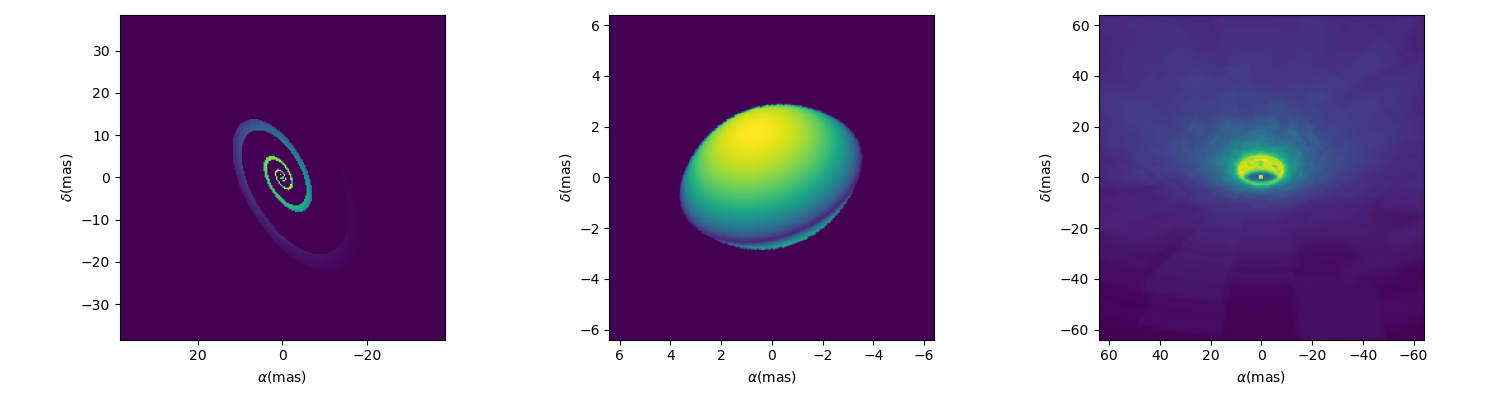
The first one is a spiral implemented as oimSpiral.

Its implementation is descrbided in details in the section Image plane component from simple formula (Spiral).

spiral = oim.oimSpiral(dim=256, fwhm=20, P=0.1, width=0.2, pa=30, elong=2)
mspiral = oim.oimModel(spiral)

The second one is a simple simulation of a fast-rotator using the Roche model and a beta-law gravity-darkening. It is implemented in oimodeler as oimFastRotator and a full description is given in Image-plane component from external code (Fast Rotator).

frot = oim.oimFastRotator(dpole=5, dim=128, incl=-50,rot=0.99, Tpole=20000, beta=0.25,pa=20)
mfrot = oim.oimModel(frot)

Finally, the last one is an output from the radiative transfer code RADMC3D simulating the inner part of a dusty disk around the B[e] star FS CMa. The simulation was made from 1.5 to 13μm. and the output was saved as a chromatic image-cube in the fits format with proper axes descruibed in the header (size of pixel in x, y and wavelength). We use the oimComponentFitsImage class described in the next section to load the image as a image-components.

radmc3D_fname = product_dir / "radmc3D_model.fits"
radmc3D = oim.oimComponentFitsImage(radmc3D_fname,pa=180)
mradmc3D = oim.oimModel(radmc3D)

Unlike when using Fourier-based components, the determination of the complex coherent flux (and the other interferometric observables) from an image requires the computation of the image Fourier Transform (FT) at the spatial frequency (and optionnally spectral and time) coordinates of the data.

In oimodeler such computation relies on the oimFTBackends module which contains various algorithms to compute the Fourier trasnform. Currently implemented are the following:

Available Fourier Transform Backends

class name	Alias	Description
numpyFFTBackend	numpyfft	2D FFT with 4D interpolation using the numpy.fft (precision depends on the padding parameter)
FFTWBackend	fftw	2D FFT with 4D interpolation using the pyFFTW package (precision depend on the padding parameter)
DFTBackend	DFT	Discreet Fourier Transform a the correct spatial frequency (2D interpolation possible between wavelengths and time)

By default the standard numpy FFT backend will be used. The FFTW backend which is significantly faster can be actived if pyFFTW is installed on your system. To check which backend is available on your installation, type:

print(oim.oimOptions.ft.backend.available)

[<class 'oimodeler.oimFTBackends.numpyFFTBackend'>,
 <class 'oimodeler.oimFTBackends.FFTWBackend'>]

The current FT backend is given by :

print(oim.oimOptions.ft.backend.active)

<class 'oimodeler.oimFTBackends.numpyFFTBackend'>

To change it you can modify directly oimOptions namespace:

oim.oimOptions.ft.backend.active = oim.FFTWBackend

Or you can use the FT backend alias with the function setFTBackend

oim.setFTBackend("fftw")

The FFT backends (numpy or FFTW) are significantly faster than a normal DFT, but its precision depends on the zero-padding of the image. The default zero padding factor is set to 4 which means the the the image will be zero-padded in a 4 times bigger array (rounded to the closest power of 2). The user can access and change the zero padding using the oimOptions namespace :

oim.oimOptions.ft.padding = 8

Depending on the sharpness of the object image and its cropping lowering the zero-padding might lead to important errors.

Here is a ample script illustrating the accuracy of the FFT as the function of the padding factor using the oimSpiral component as example.

#creating the spiral model
spiral = oim.oimSpiral(dim=128, fwhm=20, P=1, width=0.1, pa=0, elong=1)
mspiral = oim.oimModel(spiral)

#creating a set of baselines from 0 to 100m in K band
wl = 2.1e-6
B = np.linspace(0, 100, num=200)
spf = B/wl

#computing the reference model with padding of 32
oim.oimOptions.ft.padding = 32
ccf01 = mspiral.getComplexCoherentFlux(spf, spf*0)
v01 = np.abs(ccf01/ccf01[0])

start = time.time()
ccf02 = mspiral.getComplexCoherentFlux(spf*0, spf)
v02 = np.abs(ccf02/ccf02[0])
end = time.time()
dt0 = end -start

#%%  computing FFT with different padding
padding=[16,8,4,2,1]
figpad,axpad = plt.subplots(2,2, figsize=(10,5),sharey="row",sharex=True)

axpad[0,0].plot(spf, v01, color="k",lw=4)
axpad[0,1].plot(spf, v02, color="k",lw=4,label=f"padding=32x ({dt0*1000:.0f}ms)")

for pi in padding :
    oim.oimOptions.ft.padding = pi
    ccf1 = mspiral.getComplexCoherentFlux(spf, spf*0)
    v1 = np.abs(ccf1/ccf1[0])
    start = time.time()
    ccf2 = mspiral.getComplexCoherentFlux(spf*0, spf)
    v2 = np.abs(ccf2/ccf2[0])
    end = time.time()
    dt = end -start
    axpad[0,0].plot(spf, v1)
    axpad[0,1].plot(spf, v2,label=f"padding={pi}x ({dt*1000:.0f}ms)")
    axpad[1,0].plot(spf, (v1-v01)/v01*100,marker=".",ls="")
    axpad[1,1].plot(spf, (v2-v02)/v02*100,marker=".",ls="")

for i in range(2):
    axpad[1,i].set_xlabel("spatial frequency (cycles/rad)")
    axpad[1,i].set_yscale("symlog")
axpad[0,0].set_title("East-West baselines")
axpad[0,1].set_title("North-South baselines")
axpad[0,0].set_ylabel("Visbility")
axpad[0,1].legend()
axpad[1,0].set_ylabel("Residual (%)")

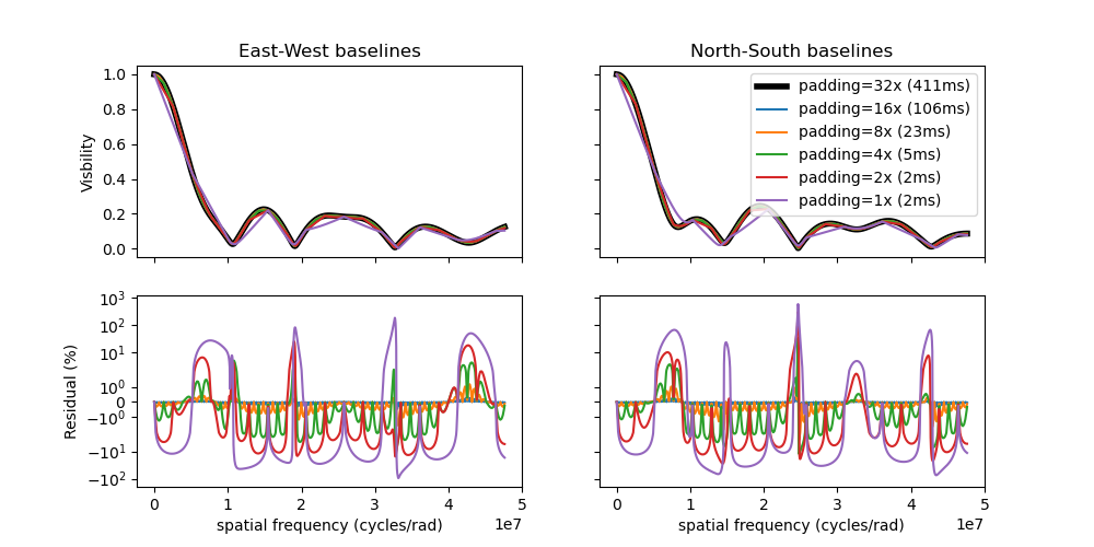
In the case of the oimSpiral component, reducing the zero-padding below the default value of 4 leads to mean errors of the order of 30% (with values up to 500%). The default padding reduce mean errors to a few percents (with maximum of the order of 10%).

However, as the FFT computation time grows like \(n log(n)\), where n is the number of pixels in the image, increasing the padding increase significantly the computation time of the model (see the example above).

Another way to reduce the computation time of the FFT (and the DFT) is to reduce the size of the image and increase the pixel size of the image while keeping the field of view fixed.

Finally, when dealing with image-component, the user show determine the good trade-off between image resolution and size, zero-padding and computation time.

Loading fits images

One special and very useful image based component is the oimComponentFitsImage that allows the loading precomputed images and use them as normal oimodeler components.

To illustrate the functionalities of this component we will use two fits files representing a classical Be star and its circumstellar disk:

1. a H-band continuum image generated using the DISCO semi-physical code as described in Vieira et al. (2015)

2. a chromatic image-cube computed around the \(Br\,\gamma\) emission line using the Kinematic Be disk model as described in Meilland et al. (2012)

Note

Both models were generated using the AMHRA service of the JMMC.

AMHRA develops and provides various astrophysical models online, dedicated to the scientific exploitation of high-angular and high-spectral facilities. Currently available models are:

• Semi-physical gaseous disk of classical Be stars and dusty disk of YSO.

• Red-supergiant and AGB.

• Binary spiral for WR stars.

• Physical limb darkening models.

• Kinematics gaseous disks.

• A grid of supergiant B[e] stars models.

Monochromatic image

The code corresponding to this section is available in LoadingFitsImage.py

The fits-formatted image BeDisco.fits that we will use is located in oimodeler data\IMAGES directory.

There are two ways to load a fits image into a oimComponentFitsImage object. The first one is to open the fits file using the astropy.io.fits module of the astropy package and then passing it to the oimComponentFitsImage class.

im = fits.open(file_name)
c = oim.oimComponentFitsImage(im)

However, if the user doesn’t need to directly access the content of the image, the filename can be passed directly to the oimComponentFitsImage class.

c = oim.oimComponentFitsImage(file_name)

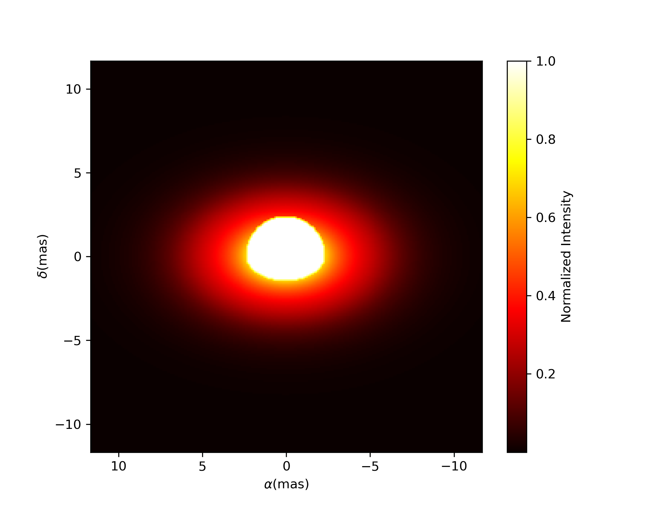
Finally, we can build our model with this unique component and plot the model image with an arbitrary pixel size and dimension:

m = oim.oimModel(c)
m.showModel(512, 0.05, legend=True, normalize=True, normPow=1, cmap="hot")

When using the image-component, the image shown by the showModel method is interpolated and crop or zero-padded depending on the internal image dimension and pixel size and the dimension and pixel size used in the showModel method.

One can retrieve the component internal image (the one loaded from the fits file) using the ._internalImage() function

im_disco = cdisco._internalImage()
print(im_disco.shape)

(1, 1, 256, 256)

The first two dimensions are the time and the wavelength but they are 1 as our model is static and grey.

Note

The internal image can be modify that way if needed.

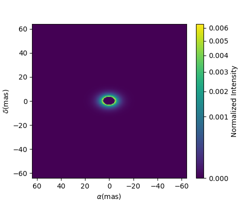
The internal pixel size in rad can also be retrieved using the `_pixSize variable. This can be used to plot the image using the showModel method without rescaling. Here we use astropy.units to convert the radians in mas.

import astropy.units as u
pixSize = cdisco._pixSize*u.rad.to(u.mas)
dim = im_disco.shape[-1]
mdisco.showModel(dim, pixSize, legend=True, normalize=True, normPow=1, cmap="hot")

We now create spatial frequencies for a thousand baselines ranging from 0 to 120 m, in the North-South and East-West orientation and at an observing wavlength of 1.5 microns.

wl, nB = 1.5e-6, 1000
B = np.linspace(0, 120, num=nB)

spfx = np.append(B, B*0)/wl # 1st half of B array are baseline in the East-West orientation
spfy = np.append(B*0, B)/wl # 2nd half are baseline in the North-South orientation

We compute the complex coherent flux and then the absolute visibility

ccf = m.getComplexCoherentFlux(spfx, spfy)
v = np.abs(ccf)
v = v/v.max()

and, finally, we can plot our results:

plt.figure()
plt.plot(B , v[0:nB],label="East-West")
plt.plot(B , v[nB:],label="North-South")
plt.xlabel("B (m)")
plt.ylabel("Visbility")
plt.legend()
plt.margins(0)

Let’s now have a look at the model’s parameters:

pprint(m.getParameters())

... {'c1_Fits_Comp_dim': oimParam at 0x19c6201c820 : dim=128 ± 0  range=[1,inf] free=False ,
     'c1_Fits_Comp_f': oimParam at 0x19c6201c760 : f=1 ± 0  range=[0,1] free=True ,
     'c1_Fits_Comp_pa': oimParam at 0x19c00b9bbb0 : pa=0 ± 0 deg range=[-180,180] free=True ,
     'c1_Fits_Comp_scale': oimParam at 0x19c6201c9d0 : scale=1 ± 0  range=[-inf,inf] free=True ,
     'c1_Fits_Comp_x': oimParam at 0x19c6201c6a0 : x=0 ± 0 mas range=[-inf,inf] free=False ,
     'c1_Fits_Comp_y': oimParam at 0x19c6201c640 : y=0 ± 0 mas range=[-inf,inf] free=False }

In addition to the x, y, and f parameters, common to all components, the oimComponentFitsImage have three additional parameters:

• dim: The fixed size of the internal fits image (currently only square images are compatible).

• pa: The position of angle of the component (used for rotating the component).

• scale: A scaling factor for the component.

The position angle pa and the scale are both free parameters (as default) and can be used for model fitting.

Let’s try to rotate and scale our model and plot the image again.

c.params['pa'].value = 45
c.params['scale'].value = 2
m.showModel(256, 0.04, legend=True, normPow=0.4, colorbar=False)

The oimComponentFitsImage can be combined with any kind of other component. Let’s add a companion (i.e., uniform disk) for our Be star model.

c2 = oim.oimUD(x=20, d=1, f=0.03)
m2 = oim.oimModel(c, c2)

We add a 1 mas companion located at 20 mas East of the central object with a flux of 0.03. We can now plot the image of our new model.

m2.showModel(256, 0.2, legend=True, normalize=True, fromFT=True, normPow=1, cmap="hot")

To finish this example, let’s plot the visibility along North-South and East-West baseline for our binary Be-star model.

ccf = m2.getComplexCoherentFlux(spfx, spfy)
v = np.abs(ccf)
v = v/v.max()

plt.figure()
plt.plot(B, v[0:nB], label="East-West")
plt.plot(B, v[nB:], label="North-South")
plt.xlabel("B (m)")
plt.ylabel("Visbility")
plt.legend()
plt.margins(0)

Using a chromatic image-cube

The oimComponentFitsImage can also be used to import fits files containing chromatic image-cubes into oimodeler.

In this example we will use a chromatic image-cube computed around the \(Br\,\gamma\) emission line for a classical Be star circumstellar disk. The model, detailed in Meilland et al. (2012) was computed using the AMHRA service of the JMMC.

The fits-formatted image-cube we will use, KinematicsBeDiskModel.fits, is located in the data/IMAGES directory.

The code corresponding to this section is available in LoadingFitsImageCube.py

We build our chromatic model the same way as for a monochromatic image.

c = oim.oimComponentFitsImage(file_name)
m = oim.oimModel(c)

However, unlike for the monochromatic image, our model is now chromatic. The internal image-cube can be accessed through the private variable c._image of the oimComponentFitsImage and the wavelength table using _wl

print(c._image.shape)
print(c._wl)

(1, 25, 256, 256)
[2.16286e-06 2.16313e-06 2.16340e-06 2.16367e-06 2.16394e-06 2.16421e-06
 2.16448e-06 2.16475e-06 2.16502e-06 2.16529e-06 2.16556e-06 2.16583e-06
 2.16610e-06 2.16637e-06 2.16664e-06 2.16691e-06 2.16718e-06 2.16745e-06
 2.16772e-06 2.16799e-06 2.16826e-06 2.16853e-06 2.16880e-06 2.16907e-06
 2.16934e-06]

The image-cube contains 256x256 pixels images at 25 wavelength ranging from 2.16286 to 2.16934:math:`mu`m.

We can now plot some images through the \(Br\gamma\) emission line (21661 \(\mu`m)using the :func:`oimModel.showModel <oimodeler.oimModel.oimModel.showModel>\) method. We need to specify some wavelengths. Images will be interpolated between the internal image-cubve wavelengths.

wl0, dwl, nwl = 2.1661e-6, 60e-10, 5
wl = np.linspace(wl0-dwl/2, wl0+dwl/2, num=nwl)
fig, ax, im  = m.showModel(256, 0.04, wl=wl, legend=True, normPow=0.4,colorbar=False)

Here is a small piece of code to compute visibility for a series of 500 North-South and 500 East-West baselines ranging between 0 and 100m and with 51 wavelengths through the emission line.

nB = 1000
nwl = 51

wl = np.linspace(wl0-dwl/2, wl0+dwl/2, num=nwl)
B = np.linspace(0, 100, num=nB//2)

# The 1st half of B array are baseline in the East-West orientation
# and the 2nd half are baseline in the North-South orientation
Bx = np.append(B, B*0)
By = np.append(B*0, B)

#creating the spatial frequencies and wls arrays nB x nwl by matrix multiplication
spfx = (Bx[np.newaxis,:]/wl[:,np.newaxis]).flatten()
spfy = (By[np.newaxis,:]/wl[:,np.newaxis]).flatten()
wls  = (wl[:,np.newaxis]*np.ones([1,nB])).flatten()

#computing the complex coherent flux and visbility
vc = m.getComplexCoherentFlux(spfx, spfy, wls)
v = np.abs(vc.reshape(nwl, nB))
v = v/np.tile(v[:, 0][:, None], (1, nB))

#plotting the results
fig, ax = plt.subplots(1, 2, figsize=(8, 4))
titles = ["East-West Baselines", "North-South Baselines"]

for iB in range(nB):
    cB = (iB % (nB//2))/(nB//2-1)
    ax[2*iB//nB].plot(wl*1e9, v[:, iB],
                      color=plt.cm.plasma(cB))

for i in range(2):
    ax[i].set_title(titles[i])
    ax[i].set_xlabel(r"$\lambda$ (nm)")
ax[0].set_ylabel("Visibility")
ax[1].get_yaxis().set_visible(False)

norm = colors.Normalize(vmin=np.min(B), vmax=np.max(B))
sm = cm.ScalarMappable(cmap=plt.cm.plasma, norm=norm)
fig.colorbar(sm, ax=ax, label="B (m)")

As expected, for a rotating disk (see Meilland et al. (2012) for more details), the visibility for the baselines along the major-axis show a W-shaped profile through the line, whereas the visibliity along the minor-axis of the disk show a V-shaped profile.

Radial-Profile components

Warning

oimodeler radial profile component is not yet fully tested. Use at your own risk!

Although not fully implemented and optimize, oimodeler allow to use 1D intensity radial profile for circular or intensity distributions. Radial-profile components are derived from the semi-abstract class oimComponentRadialProfile .This class implement complex-coherent-flux computation using Hankel transform which take into account flattening for elliptic components.

The code corresponding to this section is available in radialProfileComponents.py

Here is the list of radial-profile components currently implemented in oimodeler

Available radial profile components

Component Name	Short description	Parameters
oimComponentRadialProfile	Generic component	x, y, f, dim
oimExpRing	Exponential Ring	x, y, f, elong, pa, dim, d, fwhm
oimRadialRing	Radial Ring	x, y, f, elong, pa, dim, din, dout, p
oimRadialRing2	Radial Ring2	x, y, f, dim, din, w, p
oimTempGrad	Temperature Gradient	x, y, f, elong, pa, dim, rin, rout, r0, temp0, dust_mass, q, p, kappa_abs, dist

You can get this list using the listComponents function.

print(oim.listComponents(componentType="radial"))

['oimComponentRadialProfile', 'oimExpRing', 'oimRadialRing',
 'oimRadialRing2', 'oimTempGrad', 'oimAsymTempGrad']

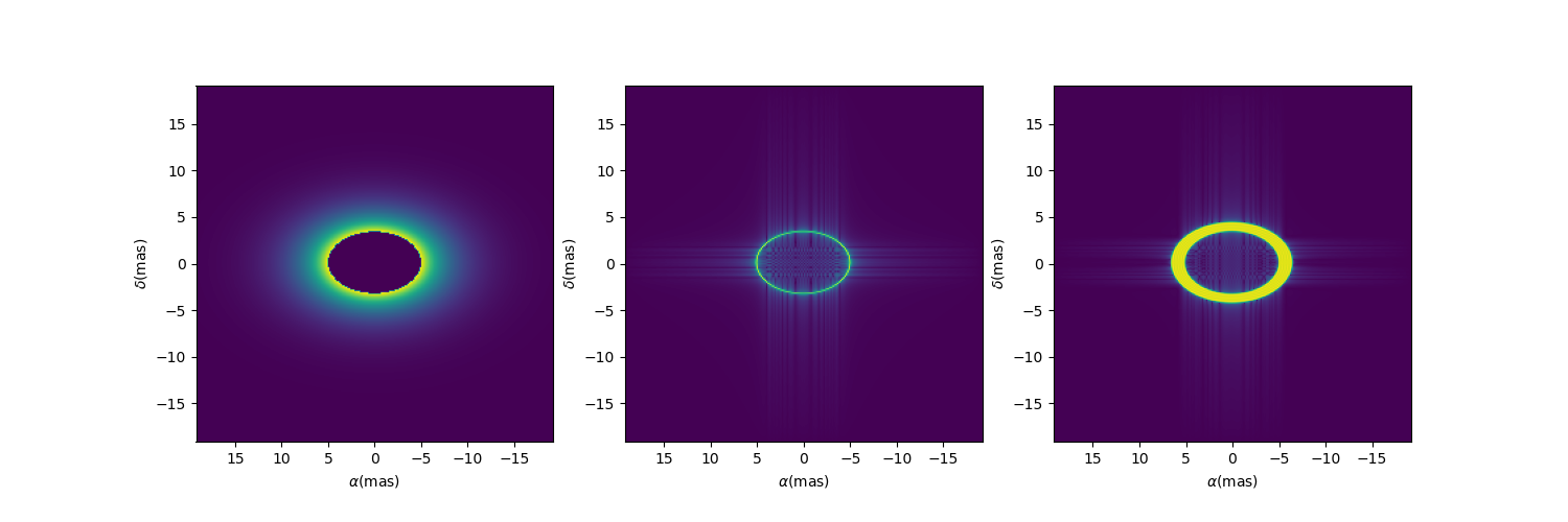
Let’s build a model with the exponential ring.

c = oim.oimExpRing(d=10,fwhm=1,elong=1.5,pa=90)
m = oim.oimModel(c)
fig, ax, im = m.showModel(256,0.5)

Let’s compare the visibility from this model to that of two other rings defined using the Fourier-based components:

• a 10 mas infinitesimal ring

• a 10 mas uniform ring with a 5 mas width

c1 = oim.oimIRing(d=10,elong=1.5,pa=90)
m1 = oim.oimModel(c1)

c2 = oim.oimRing(din=10,dout=13,elong=1.5,pa=90)
m2 = oim.oimModel(c2)

fig, ax = plt.subplots(1,3,figsize=(15,5))

m.showModel(256,0.15,figsize=(5,4),axe=ax[0],colorbar=False)
m1.showModel(256,0.15,figsize=(5,4),axe=ax[1],fromFT=True,colorbar=False)
m2.showModel(256,0.15,figsize=(5,4),axe=ax[2],fromFT=True,colorbar=False)

We will simulated visibilities for 1000 East-West baselines in the K-band.

wl = 2.1e-6
B = np.linspace(0, 100, num=10000)
spf = B/wl

start = time.time()
ccf = m.getComplexCoherentFlux(spf, spf*0)
v = np.abs(ccf/ccf[0])
dt = (time.time() - start)*1000


start = time.time()
ccf1 = m1.getComplexCoherentFlux(spf, spf*0)
v1 = np.abs(ccf1/ccf1[0])
dt1 = (time.time() - start)*1000

start = time.time()
ccf2 = m2.getComplexCoherentFlux(spf, spf*0)
v2 = np.abs(ccf2/ccf2[0])
dt2 = (time.time() - start)*1000

plt.figure()
plt.plot(B, v, label=f"Exponential Ring ({dt:.1f}ms)")
plt.plot(B, v1, label=f"Infinitesimal Ring ({dt1:.1f}ms)")
plt.plot(B, v2, label=f"Uniform Ring ({dt2:.1f}ms)")
plt.xlabel("B (m)")
plt.ylabel("Visbility")
plt.legend()
plt.margins(0)

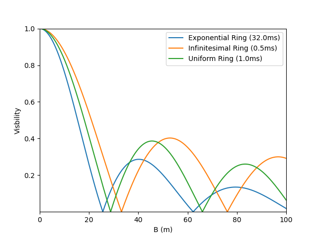
Note

Remember that, as for Image-based model, the computation time of visibility from radial profiles is much longer than that of the basic Fourier-based components as show in the figure above.

Parameter interpolators

Here we present in more details the parameter

interpolators. This example can be found in the paramInterpolators.py script.

The following table summarize the available interpolators and their parameters. Most of them will be presented in this example.

Available parameter interpolators

Class Name	oimInterp macro	Description	parameters
oimParamInterpolator		Generic interpolator (to be subclassed)
oimParamInterpolatorKeyframes		Interpolation between keyframes in wl or mjd	keyframes, keyvalues, kind, dependence, fixedRef, extrapolate
oimParamInterpolatorWl	wl	Interpolation between keyframes in wl	wl, values, kind, fixedRef, extrapolate
oimParamInterpolatorTime	time	Interpolation between keyframes in mjd	mjd, values, kind, fixedRef, extrapolate
oimParamCosineTime	cosTime	Assymetrical cosine time interpolator	T0, P, values, x0
oimParamGaussian		Generic gaussian interpolator in wl or mjd	dependence, val0, value, x0, fwhm
oimParamGaussianWl	GaussWl	Gaussian interpolator in wl	val0, value, x0, fwhm
oimParamGaussianTime	GaussTime	Gaussian interpolator in mjd	val0, value, x0, fwhm
oimParamMultipleGaussian		Generic multiple gaussian interpolator in wl or mjd	dependence, val0, values, x0, fwhm
oimParamMultipleGaussianWl	mGaussWl	Multiple Gaussian interpolator in wl	val0, values, x0, fwhm
oimParamMultipleGaussianTime	mGaussTime	Multiple Gaussian interpolator in mjd	val0, values, x0, fwhm
oimParamPolynomial		Generic polynomial interpolation in wl or mjd	dependence, order, coeffs, x0
oimParamPolynomialWl	polyWl	Polynomial interpolation in wl	order, coeffs, x0
oimParamPolynomialTime	polyTime	Polynomial interpolation in mjd	order, coeffs, x0
oimParamPowerLaw		Powerlaw interpolation in wl or mjd	dependence, x0, A, p
oimParamPowerLawTime	powerlawTime	Powerlaw interpolation in mjd	x0, A, p
oimParamPowerLawWl	powerlawWl	Powerlaw interpolation in wl	x0, A, p
oimParamLinearRangeWl	rangeWl	Linear range interpolation in wl	wlmin, wlmax, values
oimParamLinearTemplateWl	templateWl	Interpolation in wl using external regular grid template	wl0, dwl, f_contrib, values, kind
oimParamLinearTemperatureWl	tempWl	Blackbody in wl for given temperature	temp, solid_angle
oimParamLinearStarWl	starWl	Blackbody in wl for given Teff, dist, and radius or lum	temp, dist, lum, radius
oimParamUserFunc	userFunc	Interpolate from user-supplied function

In order to simplify plotting the various interpolators we define a plotting function that can works for either a chromatic or a time-dependent model. With some baseline length, wavelength, time vectors passed and some model and interpolated parameter, the function will plot the interpolated parameters as a function of the wavelength or time, and the corresponding visibilities.

def plotParamAndVis(B, wl, t, model, param, ax=None, colorbar=True):
    nB = B.size

    if t is None:
        n = wl.size
        x = wl*1e6
        y = param(wl, 0)
        xlabel = r"$\lambda$ ($\mu$m)"
    else:
        n = t.size
        x = t-60000
        y = param(0, t)
        xlabel = "MJD - 60000 (days)"

    Bx_arr = np.tile(B[None, :], (n, 1)).flatten()
    By_arr = Bx_arr*0

    if t is None:
        t_arr = None
        wl_arr = np.tile(wl[:, None], (1, nB)).flatten()
        spfx_arr = Bx_arr/wl_arr
        spfy_arr = By_arr/wl_arr
    else:
        t_arr = np.tile(t[:, None], (1, nB)).flatten()
        spfx_arr = Bx_arr/wl
        spfy_arr = By_arr/wl
        wl_arr = None

    v = np.abs(model.getComplexCoherentFlux(
        spfx_arr, spfy_arr, wl=wl_arr, t=t_arr).reshape(n, nB))

    if ax is None:
        fig, ax = plt.subplots(2, 1)
    else:
        fig = ax.flatten()[0].get_figure()

    ax[0].plot(x, y, color="r")

    ax[0].set_ylabel("{} (mas)".format(param.name))
    ax[0].get_xaxis().set_visible(False)

    for iB in range(1, nB):
        ax[1].plot(x, v[:, iB]/v[:, 0], color=plt.cm.plasma(iB/(nB-1)))

    ax[1].set_xlabel(xlabel)
    ax[1].set_ylabel("Visibility")

    if colorbar == True:
        norm = colors.Normalize(vmin=np.min(B[1:]), vmax=np.max(B))
        sm = cm.ScalarMappable(cmap=plt.cm.plasma, norm=norm)
        fig.colorbar(sm, ax=ax, label="Baseline Length (m)")

    return fig, ax, v

We will need a baseline length vector (here 200 baselines between 0 and 60m) and we will build for each model either a length 1000 wavelength or time vector.

nB = 200
B = np.linspace(0, 60, num=nB)

nwl = 1000
nt = 1000

Now, let’s start with our first interpolator: A Gaussian in wavelength (also available for time). It can be used to model spectral features like atomic lines or molecular bands in emission or absorption.

It has 4 parameters :

• A central wavelength x0

• A value outside the Gaussian (or offset) : val0

• A value at the maximum of the Gaussian : value

• A full width at half maximum : fwhm

To create such an interpolator, we use the class oimInterp class and specify GaussWl as the type of interpolator. In our example below we create a Uniform Disk model with a diameter interpolated between 2 mas (outside the Gaussian range) and 4 mas at the top of the Gaussian. The central wavelength is set to 2.1656 microns (Brackett Gamma hydrogen line) and the fwhm to 10nm.

c1 = oim.oimUD(d=oim.oimInterp('GaussWl', val0=2, value=4, x0=2.1656e-6, fwhm=1e-8))
m1 = oim.oimModel(c1)

Finally, we can define the wavelength range and use our custom plotting function.

wl = np.linspace(2.1e-6, 2.3e-6, num=nwl)
fig, ax, im = plotParamAndVis(B, wl, None, m1, c1.params['d'])
fig.suptitle("Gaussian interpolator in $\lambda$ on a uniform disk diameter", fontsize=10)

The parameters of the interpolator can be accessed using the params attribute of the oimParamInterpolator:

pprint(c1.params['d'].params)

... [oimParam at 0x2610e25e220 : x0=2.1656e-06 ± 0 m range=[0,inf] free=True ,
     oimParam at 0x2610e25e250 : fwhm=1e-08 ± 0 m range=[0,inf] free=True ,
     oimParam at 0x2610e25e280 : d=2 ± 0 mas range=[-inf,inf] free=True ,
     oimParam at 0x2610e25e2b0 : d=4 ± 0 mas range=[-inf,inf] free=True ]

Each one can also be accessed using their name as an attribute:

pprint(c1.params['d'].x0)

... oimParam x0 = 2.1656e-06 ± 0 m range=[0,inf] free

These parameters will behave like normal free or fixed parameters when performing model fitting. We can get the full list of parameters from our model using the getParameter method.

pprint(m1.getParameters())

... {'c1_UD_x': oimParam at 0x2610e25e100 : x=0 ± 0 mas range=[-inf,inf] free=False ,
     'c1_UD_y': oimParam at 0x2610e25e130 : y=0 ± 0 mas range=[-inf,inf] free=False ,
     'c1_UD_f': oimParam at 0x2610e25e160 : f=1 ± 0  range=[-inf,inf] free=True ,
     'c1_UD_d_interp1': oimParam at 0x2610e25e220 : x0=2.1656e-06 ± 0 m range=[0,inf] free=True ,
     'c1_UD_d_interp2': oimParam at 0x2610e25e250 : fwhm=1e-08 ± 0 m range=[0,inf] free=True ,
     'c1_UD_d_interp3': oimParam at 0x2610e25e280 : d=2 ± 0 mas range=[-inf,inf] free=True ,
     'c1_UD_d_interp4': oimParam at 0x2610e25e2b0 : d=4 ± 0 mas range=[-inf,inf] free=True }

In the dictionary returned by the getParameters method, the four interpolator parameters are called c1_UD_d_interpX.

The second interpolator presented here is the multiple Gaussian in wavelength (also available for time). It is a generalisation of the first interpolator but with multiple values for x0, fwhm and values.

c2 = oim.oimUD(f=0.5, d=oim.oimInterp("mGaussWl", val0=2, values=[4, 0, 0],
                                      x0=[2.05e-6, 2.1656e-6, 2.3e-6],
                                      fwhm=[2e-8, 2e-8, 1e-7]))
pt = oim.oimPt(f=0.5)
m2 = oim.oimModel(c2, pt)

c2.params['d'].values[1] = oim.oimParamLinker(
    c2.params['d'].values[0], "*", 3)
c2.params['d'].values[2] = oim.oimParamLinker(
    c2.params['d'].values[0], "+", -1)

wl = np.linspace(1.9e-6, 2.4e-6, num=nwl)

fig, ax, im = plotParamAndVis(B, wl, None, m2, c2.params['d'])
fig.suptitle(
    "Multiple Gaussian interpolator in $\lambda$ on a uniform disk diameter", fontsize=10)

Here, to reduce the number of free parameters of the model with have linked the second and third values of the interpolator to the first one.

Let’s look at our third interpolator: An asymmetric cosine interpolator in time. As it is cyclic it might be used to simulated a cyclic variation, for example a pulsating star.

It has 5 parameters :

• The Epoch (mjd) of the minimum value: T0.

• The period of the variation in days P.

• The mini and maximum values of the parameter as a two-elements array : value.

• Optionally, the asymmetry : x0 (x0=0.5 means no assymetry, x0=0 or 1 maximum asymmetry).

c3 = oim.oimGauss(fwhm=oim.oimInterp(
    "cosTime", T0=60000, P=1, values=[1, 3], x0=0.8))
m3 = oim.oimModel(c3)

t = np.linspace(60000, 60006, num=nt)
wl = 2.2e-6

fig, ax, im = plotParamAndVis(B, wl, t, m3, c3.params['fwhm'])
fig.suptitle(
    "Assym. Cosine interpolator in Time on a Gaussian fwhm", fontsize=10)

Now, let’s have a look at the classic wavelength interpolator (also available for time). jIt has two parameters:

• A list of reference wavelengths: wl.

• A list of values at the reference wavelengths: values.

Values will be interpolated in the range, using either linear (default), quadratic, or cubic interpolation set by the keyword kind. Outside the range of defined wavelengths the values will be either fixed (default) or extrapolated depending on the value of the extrapolate keyword.

Here, we present examples with the three kind of interpolation and with or without extrapolation.

c4 = oim.oimIRing(d=oim.oimInterp("wl", wl=[2e-6, 2.4e-6, 2.7e-6, 3e-6], values=[2, 6, 5, 6],
                                  kind="linear", extrapolate=True))
m4 = oim.oimModel(c4)
wl = np.linspace(1.8e-6, 3.2e-6, num=nwl)
fig, ax = plt.subplots(2, 6, figsize=(18, 6), sharex=True, sharey="row")

plotParamAndVis(B, wl, None, m4, c4.params['d'], ax=ax[:, 0], colorbar=False)
c4.params['d'].extrapolate = False
plotParamAndVis(B, wl, None, m4, c4.params['d'], ax=ax[:, 1], colorbar=False)

c4.params['d'].extrapolate = True
c4.params['d'].kind = "quadratic"
plotParamAndVis(B, wl, None, m4, c4.params['d'], ax=ax[:, 2], colorbar=False)
c4.params['d'].extrapolate = False
plotParamAndVis(B, wl, None, m4, c4.params['d'], ax=ax[:, 3], colorbar=False)

c4.params['d'].extrapolate = True
c4.params['d'].kind = "cubic"
plotParamAndVis(B, wl, None, m4, c4.params['d'], ax=ax[:, 4], colorbar=False)
c4.params['d'].extrapolate = False
plotParamAndVis(B, wl, None, m4, c4.params['d'], ax=ax[:, 5], colorbar=False)

plt.subplots_adjust(left=0.05, bottom=0.1, right=0.99, top=0.9,
                    wspace=0.05, hspace=0.05)
for i in range(1, 6):
    ax[0, i].get_yaxis().set_visible(False)
    ax[1, i].get_yaxis().set_visible(False)

fig.suptitle("Linear, Quadratic and Cubic interpolators (with extrapolation"
             r" or fixed values outside the range) in $\lambda$ on a uniform"
             " disk diameter", fontsize=18)

Finally, we can also use a polynominal interpolator in time (also available for wavelength). Its free parameters are the coefficients of the polynomial. The parameter x0 allows to shift the reference time (in mjd) from 0 to an arbitrary date.

c5 = oim.oimUD(d=oim.oimInterp('polyTime', coeffs=[1, 3.5, -0.5], x0=60000))
m5 = oim.oimModel(c5)

wl = 2.2e-6
t = np.linspace(60000, 60006, num=nt)

fig, ax, im = plotParamAndVis(B, wl, t, m5, c5.params['d'])
fig.suptitle(
    "Polynomial interpolator in Time on a uniform disk diameter", fontsize=10)

As for other part of the oimodeler software, oimParamInterpolator was designed so that users can easily create their own interoplators using inheritage. See the Adding a new Interpolators example.