Getting Started
You can download the complete gettingStarted
script from here.
Note
For this example we will use some OIFITS files located in the
examples/testData/ASPRO_MATISSE2
subdirectory of the oimodeler Github repository.
If you did not clone the github repository, you will need to manually download the directory containing the examples/.
These data are actually a “fake” dataset simulated with the APSRO software from the JMMC. ASPRO was used to create three MATISSE observations of a binary star with one resolved component. ASPRO allows to us to add realistic noise on the interferometric quantities.
Let’s start by importing the oimodeler package and specifiying the used
paths/directories.
from pprint import pprint
from pathlib import Path

import oimodeler as oim


path = Path(__file__).parent.parent.parent
data_dir = path / "examples" / "testData" / "ASPRO_MATISSE2"
save_dir = path / "images"
if not save_dir.exists():
    save_dir.mkdir(parents=True)

files = list(map(str, data_dir.glob("*.fits")))
If the data_dir is corretly set the files variable should be a list of paths
to three OIFITS files.
Warning
If you should try to write in a write-protected directory then python will yield
an error.
To resolve this, you can change the save_dir to another directory.
For some examples there is a second product_dir, which, in this case,
also needs to be changed.
Let’s create a simple binary model with one resolved component. It will be built using two components:
The point source has only three parameters, its coordinates x and y
(in mas by default) and it flux f. Note that all components parameters are
instances of the oimParam class. The uniform disk
has four parameters: x, y, f, and the disk diameter d which is given in mas
by default. If parameters are not set explicitly when the component is created they
are set to their default value (e.g., 0 for x, y, and d and 1 for f).
ud = oim.oimUD(d=3, f=0.5, x=5, y=-5)
pt = oim.oimPt(f=1)
We can print the description of the component easily:
pprint(ud)
... Uniform Disk x=5.00 y=-5.00 f=0.50 d=3.00
If we want the details of one of the component parameters, we can access it by
its name in the directory params of the component. For instance to access
the diameter d of the previously created uniform disk:
pprint(ud.params['d'])
... oimParam d = 3 ± 0 mas range=[-inf,inf] free
The same is possible for the x coordinate:
pprint(ud.params['x'])
... oimParam x = 5 ± 0 mas range=[-inf,inf] fixed
Note that the x parameter is fixed by default (for model fitting) whereas
the diameter d is free. The oimParam
instance also contains the unit (accessible via the oimParam.unit attribute as an
astropy.units object), uncertainties(via oimParam.error), and a range
for model fitting (via oimParam.mini for the lower and oimParam.maxi for the
upper bound).
There are various way of accessing and modifying the value of the parameter or
one of its other associated quantities (see the
basic model example
for more details).
For our example, we want to have the coordinates of the uniform disk as free parameters and set them to a range of 50 mas. We will explore a diameter between 0.01 and 20 mas and the flux between 0 and 10. On the other hand, the flux of the point source will be left to a fixed value of one.
ud.params['d'].set(min=0.01, max=20)
ud.params['x'].set(min=-50, max=50, free=True)
ud.params['y'].set(min=-50, max=50, free=True)
ud.params['f'].set(min=0., max=10.)
pt.params['f'].free = False
Finally, we can build our model consisting of these two components.
model = oim.oimModel(ud, pt)
We can print all the model’s parameters:
model.getParameters()
... {'c1_UD_x': oimParam at 0x1670462cca0 : x=5 ± 0 mas range=[-50,50] free=True,
     'c1_UD_y': oimParam at 0x1670462cac0 : y=-5 ± 0 mas range=[-50,50] free=True,
     'c1_UD_f': oimParam at 0x1670462cd60 : f=0.5 ± 0  range=[0.0,10.0] free=True,
     'c1_UD_d': oimParam at 0x1670462ca90 : d=3 ± 0 mas range=[0.01,20] free=True,
     'c2_Pt_x': oimParam at 0x1670462cc70 : x=0 ± 0 mas range=[-inf,inf] free=False,
     'c2_Pt_y': oimParam at 0x1670462cb80 : y=0 ± 0 mas range=[-inf,inf] free=False,
     'c2_Pt_f': oimParam at 0x167055de490 : f=1 ± 0  range=[-inf,inf] free=False}
Or only the free parameters:
pprint(model.getFreeParameters())
... {'c1_UD_x': oimParam at 0x167055ded30 : x=5 ± 0 mas range=[-50,50] free=True,
     'c1_UD_y': oimParam at 0x167055deca0 : y=-5 ± 0 mas range=[-50,50] free=True,
     'c1_UD_f': oimParam at 0x167055dec70 : f=0.5 ± 0  range=[0.0,10.0] free=True,
     'c1_UD_d': oimParam at 0x167055de850 : d=3 ± 0 mas range=[0.01,20] free=True}
Let’s now compare our data and our model. We will use the class
oimSimulator that will compute simulated
data from our model at the spatial (and optionally, spectral and temporal)
frequencies/coordinates from our data.
sim = oim.oimSimulator(data=files, model=model)
sim.compute(computeChi2=True, computeSimulatedData=True)
let’s print the \(\chi^2_r\) from our data/model comparison:
pprint("Chi2r = {}".format(sim.chi2r))
... Chi2r = 22510.099167065073
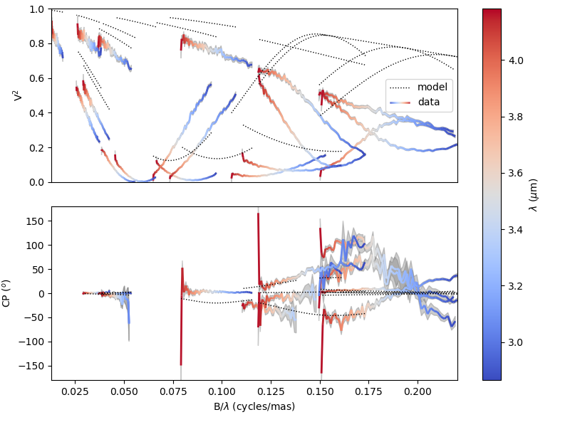
Obviously, our model is quite bad. Let’s plot a model/data comparison for the square visibility (VIS2DATA) and closure phase (T3PHI):
fig0, ax0 = sim.plot(["VIS2DATA", "T3PHI"])
The figure fig0 and axes list ax0 are returned by the oimSimulator.plot
method. You can directly save the figure using the savefig=file_name keyword.
The oimSimulator class doesn’t do
model-fitting but only data/model comparison.
To perform model-fitting we will use the oimFitterEmcee
class. This class encapsulates the famous emcee
implementation of Goodman & Weare’s Affine Invariant Markov chain Monte Carlo (MCMC)
Ensemble sampler.
Here, we create a simple emcee fitter with 10 independent walkers.
We can either give the fitter a oimSimulator
class or some data (as a oimData
object or list of filenames) and a oimModel class.
fit = oim.oimFitterEmcee(files, model, nwalkers=10)
Before running the fit, we need to prepare our fitter for the mcmc run.
We choose to initialize an array of 10 walkers to a uniform random distribution
within the range given in the model parameters with min and max.
fit.prepare(init="random")
Note
An other possible option for the mcmc fitter initialization is “gaussian”.
In that case the fitter will initialize the parameters with Gaussian distributions
centered on the current value of each parameter and with a fwhm equal to its
error variable.
The initial parameters are stored in the initialParams member variable of the fitter.
pprint(fit.initialParams)
... [[30.26628081  26.02405335   7.23061417  19.19829182]
    [ 23.12647935  44.07636861   3.39149131  17.29408761]
    [ -9.311772    47.50156564   9.49185499   4.79198633]
    [-24.05134905 -12.45653228   5.36560382   0.29631924]
    [-28.13992968 -25.25330839   9.64101194   6.21004462]
    [  5.13551292  25.3735599    4.82365667   0.53696176]
    [  3.6240551  -41.03297919   4.79235224   7.12035193]
    [-10.57430397 -40.19561341   6.0687408   11.22285079]
    [ 12.76468252  16.83390367   4.40925502   5.64248841]
    [ 29.12590452  -0.20420277   4.21541399  13.16022251]]
Now we run the fit on 2000 steps. It will compute 20000 models (i.e., nsteps x
nwalkers).
fit.run(nsteps=2000, progress=True)
... 17%|█ | 349/2000 [00:10<00:48, 34.29it/s]
After the run we can plot the values of the 4 free-parameters for the 10 walkers as a function of the steps of the mcmc run.
figWalkers, axeWalkers = fit.walkersPlot()

After a few hundred steps most walkers converge to the same position having a good \(\chi^2_r\). However, from that figure will clearly see that:
Not all walkers have converged after 2000 steps.
Some walkers converge to a solution that gives significantly worse \(\chi^2\).
In optical interferometry there are often local minima in the \(\chi^2\) and it seems that some of our walkers are locked there. In our case, this minima are due to the fact that object is close be symmetrical if not for the fact than one of the component is resolved. Neverless, the \(\chi^2\) of the local minimum is about 20 times worse than the one of the global minimum.
We can plot the famous corner plot with the 1D and 2D density distributions.
For this purpose, the oimodeler package uses the corner
package.
We will discard the 1000 first steps as most of the walkers have
converged after that. By default, the corner plot also removes the data with a
\(\chi^2\) greater than 20 times those of the best model.
This option can be changed using the chi2limfact keyword in the
oimFitterEmcee.cornerPlot method.
figCorner, axeCorner = fit.cornerPlot(discard=1000)

We now can retrieve the result of our fit.
The oimFitterEmcee fitter can either
return the "best", the "mean" or the "median" model. It also returns
uncertainties estimated from the density distribution (see emcee’s
documentation for more details on the
statistics).
median, err_l, err_u, err = fit.getResults(mode='median', discard=1000)
To compute the median and mean models we use the
oimFitterEmcee.getResults method
and remove, as in the corner plot, the walkers that didn’t converge within the limit
set by the chi2limitfact keyword (default is 20).
Furthermore, we also remove the steps of the burn-in phase with the discard keyword.
When procuring the fit’s results, the simulated data with these values are also produced simultaneously in the fitter’s internal simulator. We can plot the data/model and compute the final \(\chi^2_r\).
figSim, axSim = fit.simulator.plot(["VIS2DATA", "T3PHI"])
pprint("Chi2r = {}".format(fit.simulator.chi2r))
... Chi2r = 1.0833528313932081

That’s better.
Finally, let’s plot an image of the model with the best parameters. Here, we generate
a 512x512 image with a 0.1 mas pixel size and a 0.1 power-law colorscale:
figImg, axImg, im=model.showModel(512, 0.1, normPow=0.1)
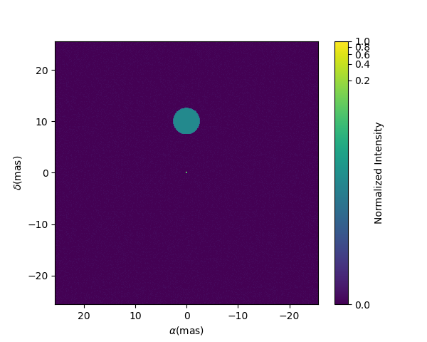
Here is our nice binary!
That’s all for this short introduction.
If you want to go further you can have a look at the Examples or API sections.