Basic Examples
In this section we presents script showing the basic functionalities
of the oimodeler software.
Loading oifits data
The exampleOimData.py
script shows how to create a oimData object from
a list of OIFITS files and how the data is organized in an
oimData instance.
from pathlib import Path
from pprint import pprint

import matplotlib.pyplot as plt
import numpy as np

import oimodeler as oim

path = Path(__file__).parent.parent.parent
data_dir = path / "examples" / "testData" / "FSCMa_MATISSE"
files = list(map(str, data_dir.glob("*.fits")))

data=oim.oimData(files)
The OIFITS data, stored in the astropy.io.fits.hdulist format, can be accessed
using the oimData.data attribute.
pprint(data.data)
... [[astropy.io.fits.hdu.image.PrimaryHDU object at 0x000002657CBD7CA0>, <astropy.io.fits.hdu.table.BinTableHDU object at 0x000002657E546AF0>, <astropy.io.fits.hdu.table.BinTableHDU object at 0x000002657E3EA970>, <astropy.io.fits.hdu.table.BinTableHDU object at 0x000002657E3EAAC0>, <astropy.io.fits.hdu.table.BinTableHDU object at 0x000002657E406520>, <astropy.io.fits.hdu.table.BinTableHDU object at 0x000002657E402EE0>, <astropy.io.fits.hdu.table.BinTableHDU object at 0x000002657E406FD0>, <astropy.io.fits.hdu.table.BinTableHDU object at 0x000002657E4600D0>],
    [<astropy.io.fits.hdu.image.PrimaryHDU object at 0x000002657E458F70>, <astropy.io.fits.hdu.table.BinTableHDU object at 0x0000026500769BE0>, <astropy.io.fits.hdu.table.BinTableHDU object at 0x000002650080EA60>, <astropy.io.fits.hdu.table.BinTableHDU object at 0x00000265007EA430>, <astropy.io.fits.hdu.table.BinTableHDU object at 0x00000265007EAAF0>, <astropy.io.fits.hdu.table.BinTableHDU object at 0x000002650080EC40>, <astropy.io.fits.hdu.table.BinTableHDU object at 0x000002657E4DC820>, <astropy.io.fits.hdu.table.BinTableHDU object at 0x000002657E4ECFD0>],
    [<astropy.io.fits.hdu.image.PrimaryHDU object at 0x000002657E4DCCA0>, <astropy.io.fits.hdu.table.BinTableHDU object at 0x0000026500B7EB50>, <astropy.io.fits.hdu.table.BinTableHDU object at 0x000002657E9F79D0>, <astropy.io.fits.hdu.table.BinTableHDU object at 0x000002657E5913A0>, <astropy.io.fits.hdu.table.BinTableHDU object at 0x000002657E591A60>, <astropy.io.fits.hdu.table.BinTableHDU object at 0x000002657E591B20>, <astropy.io.fits.hdu.table.BinTableHDU object at 0x000002657E5B7790>, <astropy.io.fits.hdu.table.BinTableHDU object at 0x000002657E5BAEB0>]]
Note
See the OIFITS standard for its conventions and the astropy.oi.fits documentation to learn how it is implemented.
To use the data efficiently in the
oimSimulator class or any of the
fitters contained in the oimFitter module
they need to be optimized in a simpler vectorial/structure.
This step is done automatically when using the simulator or fitter but can be done
manually using the following command:
data.prepareData()
For instance, this create single vectors for the data coordinates:
The u-axis of the spatial frequencies
data.vect_uThe v-axis of the spatial frequencies
data.vect_vThe wavelength data
data.vect_wl
If we now print these we can see their structure:
pprint(data.vect_u)
pprint(data.vect_v)
pprint(data.vect_wl)

pprint(data.vect_u.shape)
... [0. 0. 0. ... 0. 0. 0.]
    [0. 0. 0. ... 0. 0. 0.]
    [4.20059359e-06 4.18150239e-06 4.16233070e-06 ... 2.75303296e-06
    2.72063039e-06 2.68776785e-06]

    (5376,)
Basic models
The basicModel.py
script demonstrates the basic functionalities of the
oimModel and
oimComponents objects.
First we import the relevant packages:
from pathlib import Path
from pprint import pprint

import matplotlib.pyplot as plt
import numpy as np
import oimodeler as oim
A model is a collection of components. All components are derived from the
oimComponent class.
The components may be described in the image plane, by their intensity distribution,
or directly in the Fourier plane, for components with known analytical Fourier transforms.
In this example we will only focus on the latter type which are all derived from
the oimComponentFourier class.
In the table below is a list of the current, from the
oimComponentFourier derived,
components.
Class |
Description |
Parameters |
|---|---|---|
oimPt |
Point source |
x, y, f |
oimBackground |
Background |
x, y, f |
oimUD |
Uniform Disk |
x, y, f, d |
oimEllipse |
Uniform Ellipse |
x, y, f, d, pa, elong |
oimGauss |
Gaussian Disk |
x, y, f, fwhm |
oimEGauss |
Elliptical Gaussian Disk |
x, y, f, fwhm, pa, elong |
oimIRing |
Infinitesimal Ring |
x, y, f, d |
oimEIRing |
Elliptical Infinitesimal Ring |
x, y, f, d, pa, elong |
oimESKIRing |
Skewed Infinitesimal Elliptical Ring |
x, y, f, d, skw, skwPa, pa, elong |
oimRing |
Ring defined with din and dout |
x, y, f, din, dout |
oimERing |
Elliptical Ring with din and dout |
x, y, f, din, dout, pa, elong |
oimESKRing |
Skewed Elliptical Ring |
x, y, f, din, dout, skw, skwPa, pa, elong |
oimRing2 |
Ring defined with d and dr |
x, y, f, d, dr |
oimERing2 |
Elliptical Ring with d and dr |
x, y,f, d, dr, pa, elong |
oimLinearLDD |
Linear Limb Darkened Disk |
x, y, f, d, a |
oimQuadLDD |
Quadratic Limb Darkened Disk |
x, y, f, d, a1, a2 |
oimLorentz |
Pseudo-Lorenztian |
x, y, fwhm |
oimELorentz |
Elliptical Pseudo-Lorenztian |
x, y, f, fwhm, pa, elong |
oimConvolutor |
Convolution between 2 components |
Parameters from the 2 components |
To create models we must first create the components. Let’s create a few simple components.
pt = oim.oimPt(f=0.1)
ud = oim.oimUD(d=10, f=0.5)
g  = oim.oimGauss(fwhm=5, f=1)
r  = oim.oimIRing(d=5, f=0.5)
Here, we have create a point source components, a 10 mas uniform disk, a Gaussian distribution with a 5 mas fwhm and a 5 mas infinitesimal ring.
Note that the model parameters which are not set explicitly during the components creation are set to their default values (i.e., f=1, x=y=0).
We can print the description of the component easily:
pprint(ud)
... Uniform Disk x=0.00 y=0.00 f=0.50 d=10.00
Or if you want to print the details of a parameter:
pprint(ud.params['d'])
... oimParam d = 10 ± 0 mas range=[-inf,inf] free
Note that the components parameters are instances of the
oimParam class which hold not only the
parameter value stored in the oimParam.value attribute, but in addition to it
the following attributes:
oimParam.error: the parameters uncertainties (for model fitting).oimParam.unit: the unit as aastropy.unitsobject.oimParam.min: minimum possible value (for model fitting).oimParam.max: minimum possible value (for model fitting).oimParam.free: Describes a free parameter forTrueand a fixed parameter forFalse(for model fitting).oimParam.description: A string that describes the model parameter.
We can now create our first models using the
oimModel class.
mPt   = oim.oimModel(pt)
mUD   = oim.oimModel(ud)
mG    = oim.oimModel(g)
mR    = oim.oimModel(r)
mUDPt = oim.oimModel(ud, pt)
Now, we have four one-component models and one two-component model.
We can get the parameters of our models using the
oimModel.getParameter
method.
params = mUDPt.getParameters()
pprint(params)
... {'c1_UD_x': oimParam at 0x23de5c62fa0 : x=0 ± 0 mas range=[-inf,inf] free=False ,
     'c1_UD_y': oimParam at 0x23de5c62580 : y=0 ± 0 mas range=[-inf,inf] free=False ,
     'c1_UD_f': oimParam at 0x23de5c62400 : f=0.5 ± 0  range=[-inf,inf] free=True ,
     'c1_UD_d': oimParam at 0x23debc1abb0 : d=10 ± 0 mas range=[-inf,inf] free=True ,
     'c2_Pt_x': oimParam at 0x23debc1a8b0 : x=0 ± 0 mas range=[-inf,inf] free=False ,
     'c2_Pt_y': oimParam at 0x23debc1ab80 : y=0 ± 0 mas range=[-inf,inf] free=False ,
     'c2_Pt_f': oimParam at 0x23debc1ac10 : f=0.1 ± 0  range=[-inf,inf] free=True }
The method returns a dict of all the model component’s parameters.
The keys are defined as x{num of component}_{short Name of component}_{param name}.
Alternatively, we can get the free parameters using the
getFreeParameters method:
freeParams = mUDPt.getParameters()
pprint(freeParams)
... {'c1_UD_f': oimParam at 0x23de5c62400 : f=0.5 ± 0  range=[-inf,inf] free=True ,
     'c1_UD_d': oimParam at 0x23debc1abb0 : d=10 ± 0 mas range=[-inf,inf] free=True ,
     'c2_Pt_f': oimParam at 0x23debc1ac10 : f=0.1 ± 0  range=[-inf,inf] free=True }
The oimModel class can return an image of the
model using the oimModel.getImage method.
It takes two arguments, the image’s size in pixels and the pixel size in mas.
im = mUDPt.getImage(512, 0.1)
plt.figure()
plt.imshow(im**0.2)
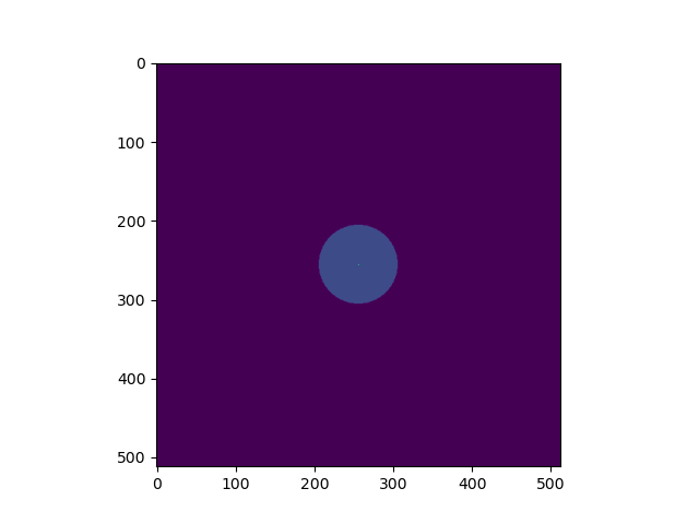
We plot the image with a 0.2 power-law to make the uniform disk components visible: Both components have the same total flux but the uniform disk is spread on many more pixels.
The image can also be returned as an astropy hdu object (instead of a numpy array)
setting the toFits keyword to True.
The image will then contained a header with the proper fits image keywords
(NAXIS, CDELT, CRVAL, etc.).
im = mUDPt.getImage(256, 0.1, toFits=True)
pprint(im)
pprint(im.header)
pprint(im.data.shape)
... <astropy.io.fits.hdu.image.PrimaryHDU object at 0x000002610B8C22E0>

SIMPLE  =                    T / conforms to FITS standard
BITPIX  =                  -64 / array data type
NAXIS   =                    2 / number of array dimensions
NAXIS1  =                  256
NAXIS2  =                  256
EXTEND  =                    T
CDELT1  = 4.84813681109536E-10
CDELT2  = 4.84813681109536E-10
CRVAL1  =                    0
CRVAL2  =                    0
CRPIX1  =                128.0
CRPIX2  =                128.0
CUNIT1  = 'rad     '
CUNIT2  = 'rad     '
CROTA1  =                    0
CROTA2  =                    0

(256, 256)
Note
Currently only regular grids in wavelength and time are allowed when exporting to fits-image format. If specified, the wl and t vectors need to be regularily sampled. The easiest way is to use the numpy.linspace function.
If their sampling is irregular an error will be raised.
Using the oimModel.saveImage method
will also return an image in the fits format and save it to the specified fits file.
im = mUDPt.saveImage("modelImage.fits", 256, 0.1)
Note
The returned image in fits format will be 2D, if time and wavelength are not specified, or if they are numbers, 3D if one of them is an array, and 4D if both are arrays.
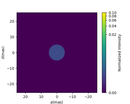
Alternatively, we can use the oimModel.showModel
method which take the same argument as the getImage, but directly create a plot with
proper axes and colorbar.
figImg, axImg = mUDPt.showModel(512, 0.1, normPow=0.2)
In other examples, we use oimModel and
oimData to create data
objects and pass them to a oimSimulator
instance to simulate interferometric quantities from the model at the spatial frequencies
from our data. Without the oimSimulator
class, the oimModel
can only produce complex coherent flux (i.e., non normalized complex visibility)
for a vector of spatial frequecies and wavelengths.
wl = 2.1e-6
B = np.linspace(0.0, 300, num=200)
spf = B/wl
Here, we have created a vector of 200 spatial frequencies, for baselines ranging from 0 to 300 m at an observing wavelength of 2.1 microns.
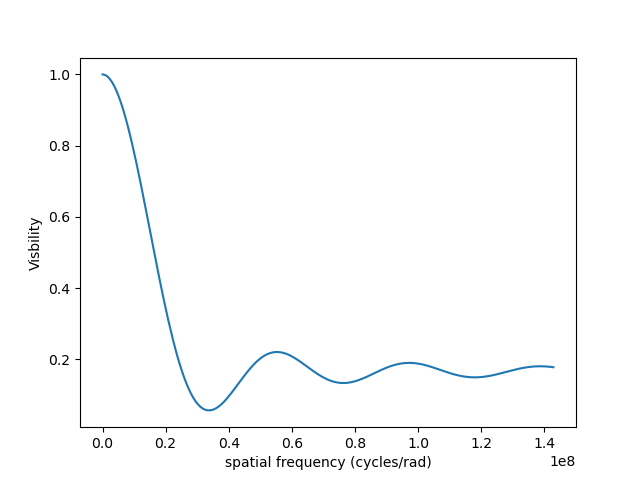
We can now use this vector to get the complex coherent flux (CCF) from our model.
ccf = mUDPt.getComplexCoherentFlux(spf, spf*0)
The oimModel.getComplexCoherentFlux
method takes four parameters: The spatial frequencies along the
East-West axis, the spatial frequencies along the North-South axis, and optionally,
the wavelength and time (mjd). Here, we are dealing with grey and
time-independent models so we don’t need to specify the wavelength. And,
as our models are circular, we don’t care about the baseline orientation.
That why we set the North-South component of the spatial frequencies to zero.
We can now plot the visibility from the CCF as the function of the spatial frequencies:
v = np.abs(ccf)
v = v/v.max()
plt.figure()
plt.plot(spf, v)
plt.xlabel("spatial frequency (cycles/rad)")
plt.ylabel("Visbility")
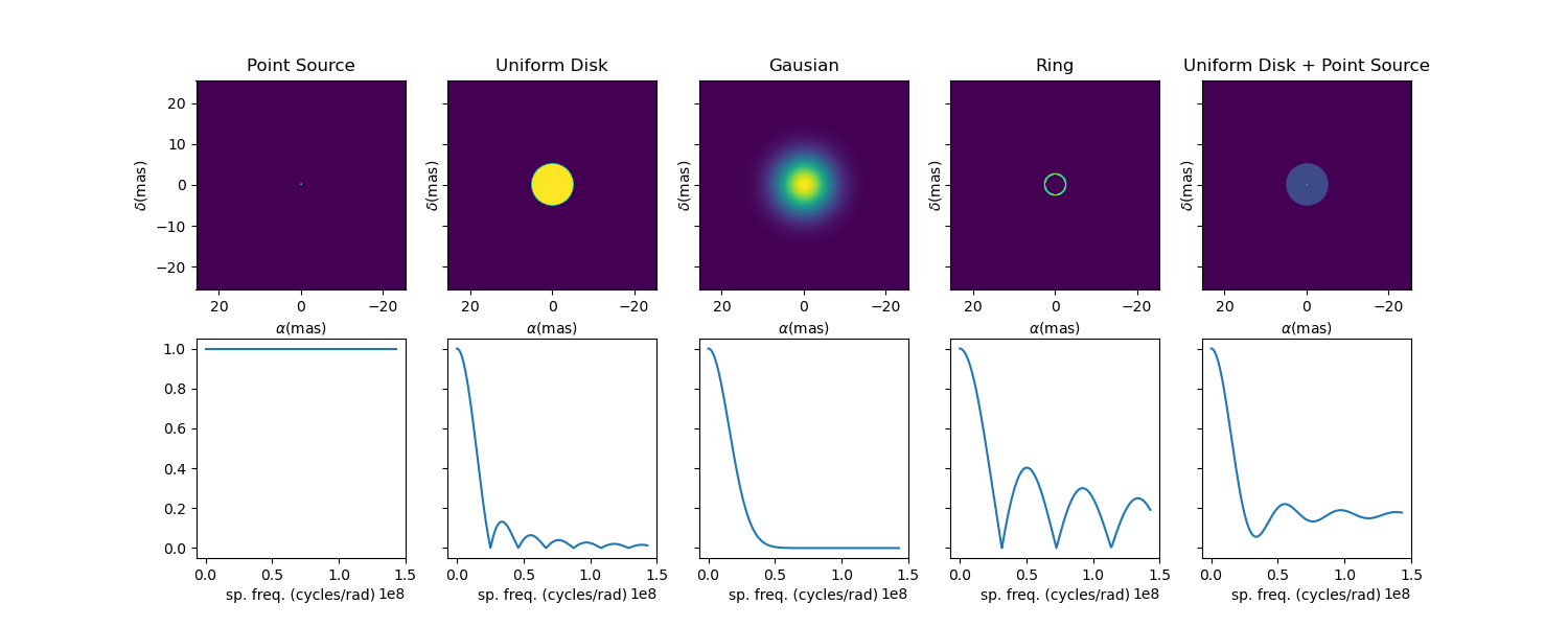
Let’s finish this example by creating a figure with the image and visibility for all the previously created models.
models = [mPt, mUD, mG, mR, mUDPt]
mNames = ["Point Source", "Uniform Disk", "Gausian", "Ring",
          "Uniform Disk + Point Source"]

fig, ax = plt.subplots(2, len(models), figsize=(
    3*len(models), 6), sharex='row', sharey='row')

for i, m in enumerate(models):
    m.showModel(512, 0.1, normPow=0.2, axe=ax[0, i], colorbar=False)
    v = np.abs(m.getComplexCoherentFlux(spf,  spf*0))
    v = v/v.max()
    ax[1, i].plot(spf, v)
    ax[0, i].set_title(mNames[i])
    ax[1, i].set_xlabel("sp. freq. (cycles/rad)")
Precomputed fits-formated image
In the FitsImageModel.py script, we demonstrate the capability of building models using precomputed image in fits format.
In this example, we will use a semi-physical model for a classical Be star and its circumstellar disk. The model, detailed in Vieira et al. (2015) was taken from the AMHRA service of the JMMC.
Note
AMHRA develops and provides various astrophysical models online, dedicated to the scientific exploitation of high-angular and high-spectral facilities.
Currently available models are:
Semi-physical gaseous disk of classical Be stars and dusty disk of YSO.
Red-supergiant and AGB.
Binary spiral for WR stars.
Physical limb darkening models.
Kinematics gaseous disks.
A grid of supergiant B[e] stars models.
Let’s start by importing oimodeler as well as useful packages.
from pathlib import Path
from pprint import pprint

import matplotlib.colors as colors
import matplotlib.cm as cm
import numpy as np
import oimodeler as oim
from matplotlib import pyplot as plt
The fits-formatted image-cube BeDisco.fits that we will use is located
in the examples/basicExamples directory.
path = Path(__file__).parent.parent.parent
file_name = path / "examples" / "BasicExamples" / "BeDISCO.fits"

save_dir = path / "images"
if not save_dir.exists():
    save_dir.mkdir(parents=True)
The class for loading fits-images and image-cubes is named
oimComponentFitsImage.
It derives from the oimComponentImage
(i.e., the partially abstract class for all components defined in the image plane).
oimComponentImage derives from the
fully abstract oimComponent (i.e. the
parent class of all oimodeler components).
Note
To learn more on the image-based models built with the oimComponent
class check the Advanced Examples and the
Expanding the Software tutorials.
There are two ways to load a fits image into a oimComponentFitsImage object.
The first one is to open the fits file using the astropy.io.fits module of the astropy
package and then passing it to the
oimComponentFitsImage
class.
im = fits.open(file_name)
c = oim.oimComponentFitsImage(im)
A simplier way, if the user doesn’t need to access directly to the content of im,
is to pass the filename to the oimComponentFitsImage
class.
c = oim.oimComponentFitsImage(file_name)
Finally, we can build our model with this unique component:
m = oim.oimModel(c)
We can now plot the model image.
m.showModel(512, 0.05, legend=True, normalize=True, normPow=1, cmap="hot")
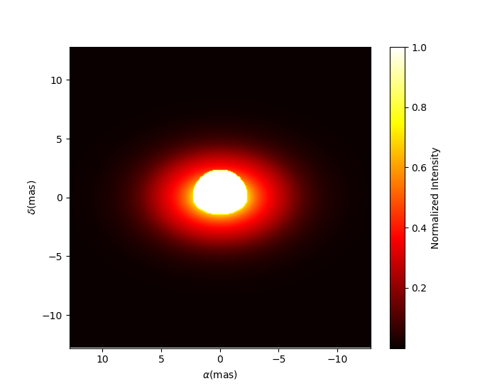
Note
Although the image was computed for a specific wavelength (i.e., 1.5 microns), our model is achromatic as we use a single image to generate it. An example with chromatic model buit on a chromatic image-cube is available here.
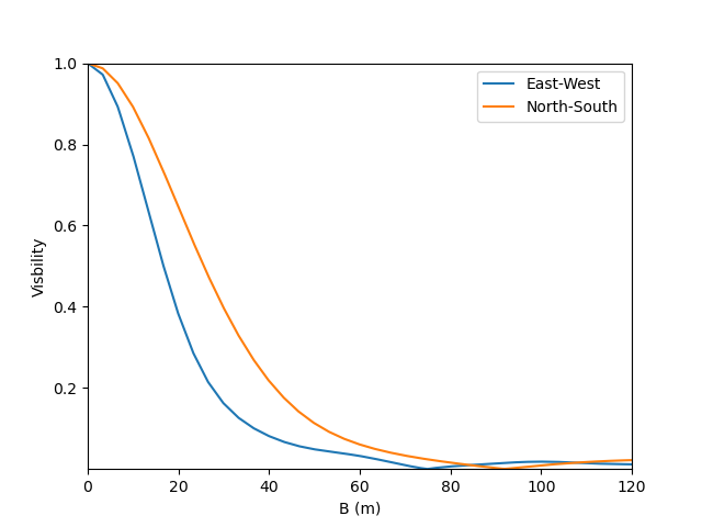
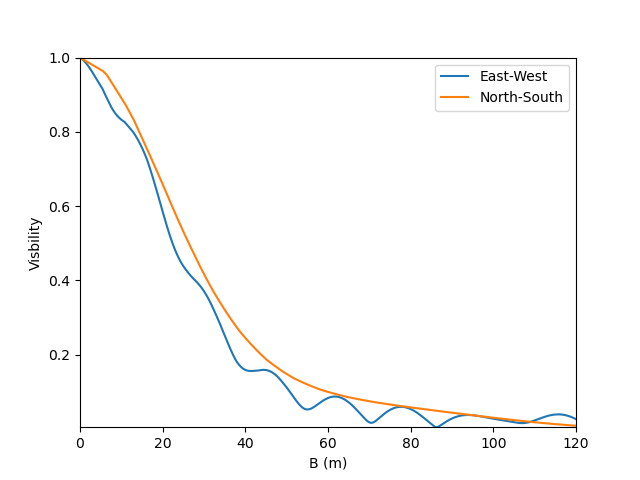
We now create spatial frequencies for a thousand baselines ranging from 0 to 120 m, in the North-South and East-West orientation and at an observing wavlength of 1.5 microns.
wl, nB = 1.5e-6, 1000
B = np.linspace(0, 120, num=nB)

spfx = np.append(B, B*0)/wl # 1st half of B array are baseline in the East-West orientation
spfy = np.append(B*0, B)/wl # 2nd half are baseline in the North-South orientation
We compute the complex coherent flux and then the absolute visibility
ccf = m.getComplexCoherentFlux(spfx, spfy)
v = np.abs(ccf)
v = v/v.max()
and, finally, we can plot our results:
plt.figure()
plt.plot(B , v[0:nB],label="East-West")
plt.plot(B , v[nB:],label="North-South")
plt.xlabel("B (m)")
plt.ylabel("Visbility")
plt.legend()
plt.margins(0)
Let’s now have a look at the model’s parameters:
pprint(m.getParameters())
... {'c1_Fits_Comp_dim': oimParam at 0x19c6201c820 : dim=128 ± 0  range=[1,inf] free=False ,
     'c1_Fits_Comp_f': oimParam at 0x19c6201c760 : f=1 ± 0  range=[0,1] free=True ,
     'c1_Fits_Comp_pa': oimParam at 0x19c00b9bbb0 : pa=0 ± 0 deg range=[-180,180] free=True ,
     'c1_Fits_Comp_scale': oimParam at 0x19c6201c9d0 : scale=1 ± 0  range=[-inf,inf] free=True ,
     'c1_Fits_Comp_x': oimParam at 0x19c6201c6a0 : x=0 ± 0 mas range=[-inf,inf] free=False ,
     'c1_Fits_Comp_y': oimParam at 0x19c6201c640 : y=0 ± 0 mas range=[-inf,inf] free=False }
In addition to the x, y, and f parameters, common to all components,
the
oimComponentFitsImage
have three additional parameters:
dim: The fixed size of the internal fits image (currently only square images are compatible).
pa: The position of angle of the component (used for rotating the component).
scale: A scaling factor for the component.
The position angle pa and the scale are both free parameters (as default) and can be used for model fitting.
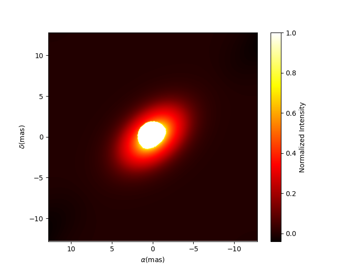
Let’s try to rotate and scale our model and plot the image again.
c.params['pa'].value = 45
c.params['scale'].value = 2
m.showModel(256, 0.04, legend=True, normPow=0.4, colorbar=False)
The oimComponentFitsImage
can be combined with any kind of other component. Let’s add a companion
(i.e., uniform disk) for our Be star model.
c2 = oim.oimUD(x=20, d=1, f=0.03)
m2 = oim.oimModel(c, c2)
We add a 1 mas companion located at 20 mas West of the central object with a flux of 0.03. We can now plot the image of our new model.
m2.showModel(256, 0.2, legend=True, normalize=True, fromFT=True, normPow=1, cmap="hot")

To finish this example, let’s plot the visibility along North-South and East-West baseline for our binary Be-star model.
ccf = m2.getComplexCoherentFlux(spfx, spfy)
v = np.abs(ccf)
v = v/v.max()

plt.figure()
plt.plot(B, v[0:nB], label="East-West")
plt.plot(B, v[nB:], label="North-South")
plt.xlabel("B (m)")
plt.ylabel("Visbility")
plt.legend()
plt.margins(0)
Data/model comparison
In the exampleOimSimulator.py
script, we use the
oimSimulator class to compare some
OIFITS data with a model.
We will compute the \(\chi^2_r\) and plot the comparison between the data an the
simulated data from the model.
Let’s start by importing the needed modules and setting the variable files to the
list of the same OIFITS files as in the Loading oifits data example.
from pathlib import Path
from pprint import pprint

import oimodeler as oim

path = Path(__file__).parent.parent.parent
data_dir = path / "examples" / "testData" / "ASPRO_MATISSE2"
save_dir = path / "images"
if not save_dir.exists():
    save_dir.mkdir(parents=True)

files = list(map(str, data_dir.glob("*.fits")))
These OIFITS were simulated with ASPRO as a MATISSE observation of a partly resolved binary star.
We make a model of a binary star where one of the components is resolved. It consists of two components: A uniform disk and a point source.
ud = oim.oimUD(d=3, f=1, x=10, y=20)
pt = oim.oimPt(f=0.5)
model = oim.oimModel([ud, pt])
We now create an
oimSimulator object and feed it
with the data and our model.
The data can either be:
A previously created
oimData.A list of previously opened astropy.io.fits.hdulist.
A list of paths to the OIFITS files (list of strings).
sim = oim.oimSimulator(data=files, model=model)
When creating the simulator, it automatically calls the oimData.prepareData
method of the created oimData instance within
the simulator instance. This calls the
oimData.prepare method of oimData
The function is used to create vectorized coordinates for the data (spatial frequencies
in x and y and wavelengths) to be passed to the oimModel
instance to compute the Complex Coherent Flux (CCF) using the
oimModel.getComplexCoherentFlux
method, and some structures to go back from the ccf to the measured interferometric
quantities contained in the OIFITS files: VIS2DATA, VISAMP, VISPHI, T3AMP, T3PHI,
and FLUXDATA.
Once the data is prepared, we can call the oimSimulator.compute
method to compute the \(\chi^2\) and the simulated data.
sim.compute(computeChi2=True, computeSimulatedData=True)
pprint("Chi2r = {}".format(sim.chi2r))
... Chi2r = 11356.162973124885
Our model isn’t fitting the data well. Let’s take a closer look and plot the data-model comparison for all interferometric quantities contained in the OIFITS files.
fig0, ax0= sim.plot(["VIS2DATA", "VISAMP", "VISPHI", "T3AMP", "T3PHI"])
You can now try to fit the model “by hand”, or go to the next example
where we use a fitter from the oimFitter
module to automatically find a good fit (and thus well fitting parameters).
Running a mcmc fit
In the exampleOimFitterEmcee.py script, we perform a complete emcee run to determine the values of the parameters of the same binary as in the (previous) Data/model comparison example.
We start by setting up the script with imports, a data list and a binary model. We don’t need to specify values for the biary parameters as they will be fitted.
from pathlib import Path
from pprint import pprint

import oimodeler as oim


path = Path(__file__).parent.parent.parent
data_dir = path / "examples" / "testData" / "ASPRO_MATISSE2"
save_dir = path / "images"
if not save_dir.exists():
    save_dir.mkdir(parents=True)

files = list(map(str, data_dir.glob("*.fits")))

ud = oim.oimUD()
pt = oim.oimPt()
model = oim.oimModel([ud,pt])
Before starting the run, we need to specify which parameters are free and what their ranges are. By default, all parameters are free, but the components x and y coordinates. For a binary, we need to release them for one of the components. As we only deal with relative fluxes, we can set the flux of one of the components to be fixed to one.
ud.params['d'].set(min=0.01, max=20)
ud.params['x'].set(min=-50, max=50, free=True)
ud.params['y'].set(min=-50, max=50, free=True)
ud.params['f'].set(min=0., max=10.)
pt.params['f'].free = False
pprint(model.getFreeParameters())
... {'c1_UD_x': oimParam at 0x23d940e4850 : x=0 ± 0 mas range=[-50,50] free=True,
     'c1_UD_y': oimParam at 0x23d940e4970 : y=0 ± 0 mas range=[-50,50] free=True,
     'c1_UD_f': oimParam at 0x23d940e4940 : f=0.5 ± 0  range=[0.0,10.0] free=True,
     'c1_UD_d': oimParam at 0x23d940e4910 : d=3 ± 0 mas range=[0.01,20] free=True}
We have 4 free-parameters, the position (x, y), the flux f and the diameter d of the uniform disk component.
Now, we can create a fitter with our model and a list of OIFITS files. We use the emcee fitter that has only one parameter, the number of walkers that will explore the parameter space.
fit = oim.oimFitterEmcee(files, model, nwalkers=32)
Note
If you are not confident with emcee, you should have a look at the documentation here.
We need to initialize the fitter using its oimFitterEmcee.prepare
method. This is setting the initial values of the walkers.
The default method is to set them to random values within the parameters’ ranges.
fit.prepare(init="random")
pprint(fit.initialParams)
... [[-37.71319618 -49.22761731   9.3299391   15.51294277]
    [-12.92392301  17.49431852   7.76169304   9.23732472]
    [-31.62470824 -11.05986877   8.71817772   0.34509237]
    [-36.38546264  33.856871     0.81935324   9.04534926]
    [ 45.30227534 -38.50625408   4.89978551  14.93004   ]
    [-38.01416866  -6.24738348   5.26662714  13.16349304]
    [-21.34600438 -14.98116997   1.20948714   8.15527356]
    [-17.14913499  10.40965493   0.37541088  18.81733973]
    [ -9.61039318 -12.02424002   6.81771974  16.22898422]
    [ 49.07320952 -34.48933488   1.75258006  19.96859116]]
We can now run the fit. We choose to run 2000 steps as a start and interactively show
the progress with a progress bar. The fit should take a few minutes on a standard computer
to compute around 64000 models (nwalkers x nsteps).
fit.run(nsteps=2000, progress=True)
The oimFitterEmcee instance stores
the emcee sampler as an attribute: oimFitterEmcee.sampler. You can, for example,
access the chain of walkers and the logrithmic of the probability directly.
sampler = fit.sampler
chain   = fit.sampler.chain
lnprob  = fit.sampler.lnprobability
We can manipulate these data. The oimFitterEmcee
implements various methods to retrieve and plot the results of the mcmc run.
The walkers position as the function of the steps can be plotted using the
oimFitterEmcee.walkersPlot
method.
figWalkers, axeWalkers = fit.walkersPlot(cmap="plasma_r")
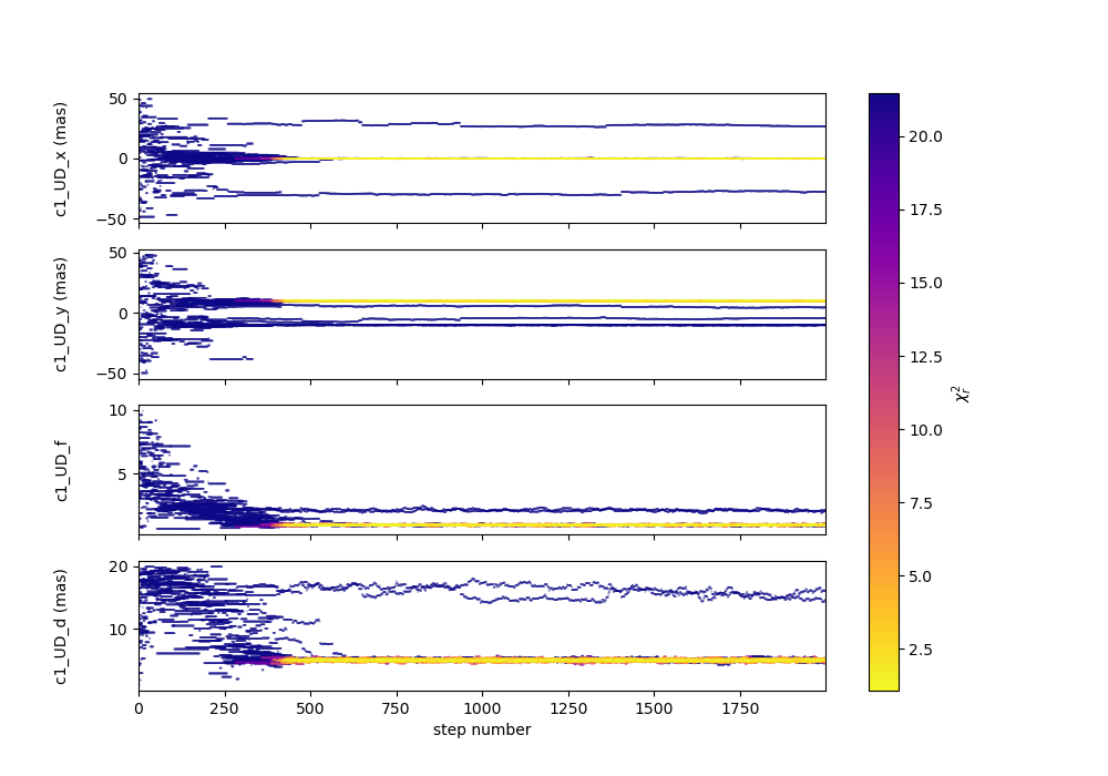
After a few hundred steps most walkers converge to a position with a good \(\chi^2_r\). However, from that figure will clearly see that:
Not all walkers have converged after 2000 steps.
Some walkers converge to a solution that gives significantly worse \(\chi^2\).
In optical interferometry there are often local minimas in the \(\chi^2\) and it seems that some of our walkers are locked in such minimas. In our case, this minimum is due to the fact that object is almost symmetrical if not for the fact than one of the component is resolved. Neverless, the \(\chi^2\) of the local minimum is about 20 times worse than the one of the global minimum.
We can plot the “famous” corner plot containing a 1D and 2D density distribution.
The oimodeler package uses the corner
library for that purpose. We will discard the first 1000 steps as most of the walkers
have converged after that. By default, the corner plot also remove the data with a \(\chi^2\)
20 times greater than those of the best model. The cutoff can be set with the
chi2limfact keyword of the oimFitter.cornerPlot
method.
figCorner, axeCorner=fit.cornerPlot(discard=1000)

We now can get the result of our fit. The
oimFitterEmcee fitter can return either
the best, the mean or the median model. It return uncertainties
estimated from the density distribution (see emcee’
for more details).
median, err_l, err_u, err = fit.getResults(mode='median', discard=1000)
To compute the median and mean model we have to remove, as in the corner plot,
the walkers that didn’t converge with the chi2limitfact keyword (default is 20)
and remove the steps of the bruning phase with the discard option.
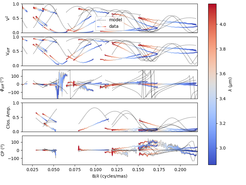
When procuring the results, the simulated data is simultaneously calculated in the fitter’s internal simulator. We can again plot the data/model and compute the final \(\chi^2_r\):
figSim, axSim=fit.simulator.plot(["VIS2DATA", "VISAMP", "VISPHI", "T3AMP", "T3PHI"])
pprint("Chi2r = {}".format(fit.simulator.chi2r))

Filtering data
Filtering can be applied to the oimData class
using the oimDataFilter class.
It is basically a stack of filters derived from the
oimDataFilterComponent
abstract class. The example presented here comes from the
exampleOimDataFilter.py
script.
As done before the required packages and create a list of the OIFITS files.
from pathlib import Path

import matplotlib.pyplot as plt
import oimodeler as oim

path = Path(__file__).parent.parent.parent
data_dir = path / "examples" / "testData" / "FSCMa_MATISSE"
save_dir = path / "images"
if not save_dir.exists():
    save_dir.mkdir(parents=True)

files = list(map(str, data_dir.glob("*.fits")))
We create an oimData object which will contain
the OIFITS data.
data = oim.oimData(files)
We now create a simple filter to cut the data to a specific wavelength range with
the oimWavelengthRangeFilter
class.
f1 = oim.oimWavelengthRangeFilter(targets="all", wlRange=[3.0e-6, 4e-6])
The oimWavelengthRangeFilter
has two keywords:
targets: Which is common to all filter components: It specifies the targeted files within the data structure to which the filter applies.Possible values are:
"all"for all files (which we use in this example).A single file specify by its index.
Or a list of indexes.
wlRange: The wavelength range to cut as a two elements list (min wavelength and max wavelength), or a list of multiple two-elements lists if you want to cut multiple wavelengths ranges simultaneously. In our example you have selected wavelength between 3 and 4 microns. Wavelengths outside this range will be removed from the data.
Now we can create a filter stack with this single filter and apply it to our data.
filters = oim.oimDataFilter([f1])
data.setFilter(filters)
By default the filter will be automatically activated as soon as a filter is set using
the oimData.setFilter method
of the oimData class.
This means that querying the oimData.data attribute will return the filtered data,
and that when using the oimData class within
an oimSimulator or an
oimFitter, the filtered data will be used
instead of the unfiltered data.
Note
The unfiltered data can always be accessed using the oimData._data attribute
and, in a similar manner, also the filtered data (that may be None if no filters
have been applied) using the private attribute oimData._filteredData.
To switch off a filter we can either call the oimData.setFilter
method without any arguments (this will remove the filter completely),
data.setFilters()
or set the useFilter attribute to False.
data.useFilter = False
Let’s plot the unfiltered and filtered data using the oimPlot
method.
fig = plt.figure()
ax = plt.subplot(projection='oimAxes')

data.useFilter = False
ax.oiplot(data, "SPAFREQ", "VIS2DATA", color="tab:blue", lw=3, alpha=0.2, label="unfiltered")

data.useFilter = True
ax.oiplot(data, "SPAFREQ", "VIS2DATA", color="tab:blue", label="filtered")

ax.set_yscale('log')
ax.legend()
ax.autolim()

Other filters for data selection are:
oimRemoveArrayFilter: Removes array(s) (such as OI_VIS, OI_T3, etc.) from the data.oimDataTypeFilter: Removes data type(s) (such as VISAMP, VISPHI, T3AMP, etc.) from the data.
Note
Actually, oimDataTypeFilter
doesn’t remove the columns with the data type from
any array as these columns are complusory in the the OIFITS format definition.
Instead, it is setting all the values of the column to zero which oimodeler
will recognize as empty for data simulation and model fitting.
f2 = oim.oimRemoveArrayFilter(targets="all", arr=["OI_VIS", "OI_FLUX"])
f3 = oim.oimDataTypeFilter(targets="all", dataType=["T3AMP"," T3PHI"])
data.setFilter(oim.oimDataFilter([f1, f2, f3]))
Here, we create a new filter stack with the previous wavelength filter f1, a filter f2 for removing the array OI_VIS and OI_FLUX from the data, and a filter f3 removing the columns T3AMP and T3PHI. Basically, we only have the VIS2DATA left in our OIFITS structure.
Note
Removing T3AMP and T3PHI from the OI_T3 is equivalent for model-fitting to removing the array OI_T3.
Plotting oifits data
Beyond the specific plots shown in the previous example, the
oimPlot module allows to plot most of the
OIFITS data in a very simple way. The example presented here comes from the
exampleOimPlot.py
script.
Let’s start by setting up the project with imports, path, and some data.
from pathlib import Path

import matplotlib.pyplot as plt
import oimodeler as oim


path = Path(__file__).parent.parent.parent
data_dir = path / "examples" / "testData" / "ASPRO_MATISSE2"
save_dir = path / "images"
if not save_dir.exists():
    save_dir.mkdir(parents=True)

files = list(map(str, data_dir.glob("*.fits")))
The oimodeler package comes with the oimAxes
class that is a subclass of the standard matplotlib.pytplot.Axes
class (the base class for all matplotlib plots). To use it, you simply need to
specify it as a projection (actually this calls the subclass) when creating
an axe or axes.
fig1 = plt.figure()
ax1 = plt.subplot(projection='oimAxes')
First, we can plot the classic uv coverage using the
oimAxes.uvplot method by passing the
list of OIFITS files (filename or opened) or an instance of a oimData
class.
ax1.uvplot(data)

We can use the oiplot method of
the oimAxes to plot any quantity inside
an OIFITS file as a function of another one. For instance, let’s plot the
squared visibilities as a function of the spatial frequencies with the wavelength
(in microns) as a colorscale.
fig2 = plt.figure()
ax2 = plt.subplot(projection='oimAxes')
lamcol=ax2.oiplot(data, "SPAFREQ", "VIS2DATA", xunit="cycles/mas", label="Data",
                  cname="EFF_WAVE", cunitmultiplier=1e6, errorbar=True)

plt.colorbar(lamcol, ax=ax2, label="$\\lambda$ ($\mu$m)")
ax2.legend()

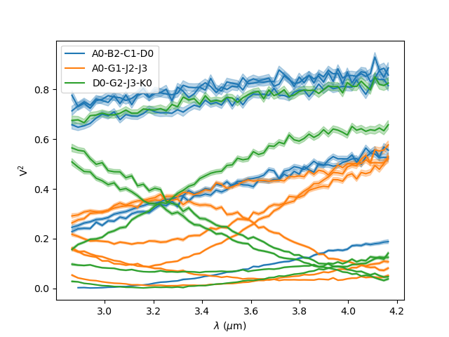
We can also plot the square visibility as the function of the wavelength while
colouring the curves by the interferometer configurations (i.e., the list of all
baselines within one file). Note that we can pass parameters to the error plots
with the kwargs_error keyword.
fig3 = plt.figure()
ax3 = plt.subplot(projection='oimAxes')
ax3.oiplot(data, "EFF_WAVE", "VIS2DATA", xunitmultiplier=1e6, color="byConfiguration",
           errorbar=True, kwargs_error={"alpha": 0.3})
ax3.legend()
Note
Special values of the color option are "byFile", "byConfiguration",
"byArrname", or "byBaseline". Other values will be interpreted as a
standard matplotlib colorname.
When using one of these values, the corresponding labels are added to the plots.
Using the oimAxes.legend method
will automatically add the proper names.
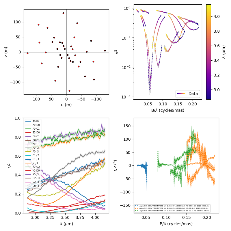
Finally, we can create a 2x2 figure with multiple plots. The projection keyword
has to be set for all oimAxes
using the subplot_kw keyword in the
matplotlib.pyplot.subplots
method.
fig4, ax4 = plt.subplots(2, 2, subplot_kw=dict(
    projection='oimAxes'), figsize=(8, 8))

ax4[0, 0].uvplot(data)

lamcol = ax4[0, 1].oiplot(data, "SPAFREQ", "VIS2DATA", xunit="cycles/mas", label="Data",
                          cname="EFF_WAVE", cunitmultiplier=1e6, ls=":", errorbar=True)

fig4.colorbar(lamcol, ax=ax4[0, 1], label="$\\lambda$ ($\mu$m)")
ax4[0, 1].legend()
ax4[1, 0].oiplot(data, "EFF_WAVE", "VIS2DATA", xunitmultiplier=1e6, color="byBaseline",
                 errorbar=True, kwargs_error={"alpha": 0.1})

ax4[1, 0].legend(fontsize=6)
ax4[1, 1].oiplot(data, "SPAFREQ", "T3PHI", xunit="cycles/mas", errorbar=True,
                 lw=2, ls=":", color="byFile")

ax4[1, 1].legend(fontsize=4)
ax4[0, 1].set_yscale('log')
ax4[1, 0].autolim()
ax4[1, 1].autolim()