Advanced Examples
Building Complex models
In the example complexModel.py we create and play with more complex Fourier-based models which includes:
Flatenning of some components
Linked parameters between components
Chromaticity of some parameters
First, we import the useful packages and create a set of spatial frequencies and wavelengths to be used to generate visibilities.
from pathlib import Path
from pprint import pprint

import numpy as np
import oimodeler as oim

fromFT = False
nB = 500  # number of baselines
nwl = 100  # number of walvengths

wl = np.linspace(3e-6, 4e-6, num=nwl)
B = np.linspace(1, 400, num=nB)
Bs = np.tile(B, (nwl, 1)).flatten()
wls = np.transpose(np.tile(wl, (nB, 1))).flatten()
spf = Bs/wls
spf0 = spf*0
Unlike in the previous example with the grey data, we create a 2D-array for the spatial
frequencies of nB baselines by nwl wavelengths. The wavlength vector is tiled
itself to have the same length as the spatial frequency vector. Finally, we flatten the
vector to be passed to the getComplexCoherentFlux method.
Let’s create our first chromatic components. Linearly chromatic parameter can added to
grey Fourier-based model by using the oimInterp
macro with the parameter "wl" when creating a new component.
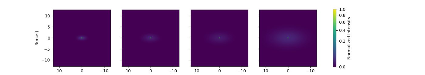
g = oim.oimGauss(fwhm=oim.oimInterp("wl" wl=[3e-6, 4e-6], values=[2, 8]))
We have created a Gaussian component with a fwhm growing from 2 mas at 3 microns
to 8 mas at 4 microns.
Note
Parameter interpolators are described in details in the following example.
We can access to the interpolated value of the parameters using the __call__
operator of the oimParam class with values
passed for the wavelengths to be interpolated:
pprint(g.params['fwhm']([3e-6, 3.5e-6, 4e-6, 4.5e-6]))
... [2. 5. 8. 8.]
The values are interpolated within the wavelength range [3e-6, 4e-6] and fixed beyond this range.
Let’s build a simple model with this component and plot the images at few wavelengths and the visibilities for the baselines we created before.
vis = np.abs(mg.getComplexCoherentFlux(
    spf, spf*0, wls)).reshape(len(wl), len(B))
vis /= np.outer(np.max(vis, axis=1), np.ones(nB))

figGv, axGv = plt.subplots(1, 1, figsize=(14, 8))
sc = axGv.scatter(spf, vis, c=wls*1e6, s=0.2, cmap="plasma")
figGv.colorbar(sc, ax=axGv, label="$\\lambda$ ($\\mu$m)")
axGv.set_xlabel("B/$\\lambda$ (cycles/rad)")
axGv.set_ylabel("Visiblity")
axGv.margins(0, 0)
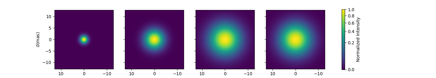
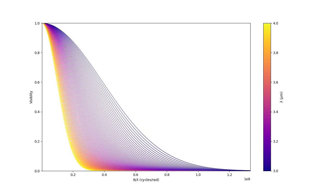
Now let’s add a second component: An uniform disk with a chromatic flux.
ud = oim.oimUD(d=0.5, f=oim.oimInterp("wl", wl=[3e-6, 4e-6], values=[2, 0.2]))
m2 = oim.oimModel([ud, g])
fig2im, ax2im, im2 = m2.showModel(256, 0.1, wl=[3e-6, 3.25e-6, 3.5e-6, 4e-6],
                                  swapAxes=True, normPow=0.2, figsize=(3.5, 2.5),
                                  fromFT=fromFT, normalize=True,
                                  savefig=save_dir / "complexModel_UDAndGauss.png")

vis = np.abs(m2.getComplexCoherentFlux(
    spf, spf*0, wls)).reshape(len(wl), len(B))
vis /= np.outer(np.max(vis, axis=1), np.ones(nB))

fig2v, ax2v = plt.subplots(1, 1, figsize=(14, 8))
sc = ax2v.scatter(spf, vis, c=wls*1e6, s=0.2, cmap="plasma")
fig2v.colorbar(sc, ax=ax2v, label="$\\lambda$ ($\\mu$m)")
ax2v.set_xlabel("B/$\\lambda$ (cycles/rad)")
ax2v.set_ylabel("Visiblity")
ax2v.margins(0, 0)
ax2v.set_ylim(0, 1)
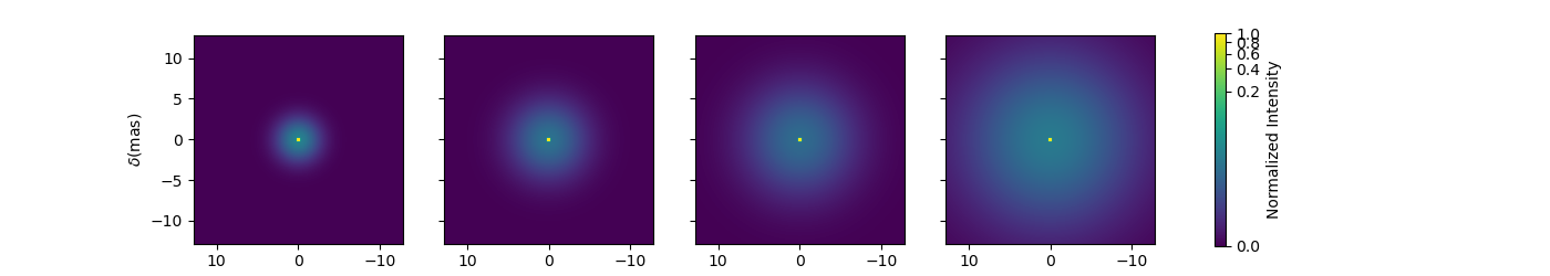
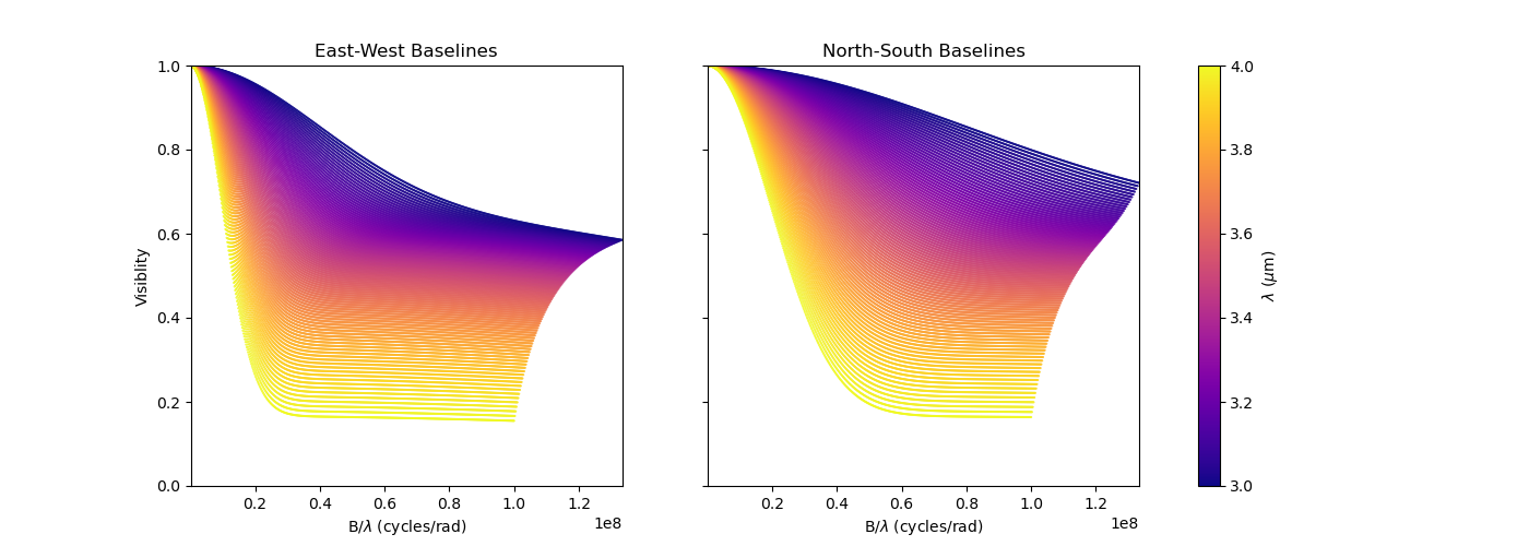
Now let’s create a similar model but with elongated components. We will replace the uniform disk by an ellipse and the Gaussian by an elongated Gaussian.
eg = oim.oimEGauss(fwhm=oim.oimInterp(
    "wl", wl=[3e-6, 4e-6], values=[2, 8]), elong=2, pa=90)
el = oim.oimEllipse(d=0.5, f=oim.oimInterp(
    "wl", wl=[3e-6, 4e-6], values=[2, 0.2]), elong=2, pa=90)

m3 = oim.oimModel([el, eg])
fig3im, ax3im, im3 = m3.showModel(256, 0.1, wl=[3e-6, 3.25e-6, 3.5e-6, 4e-6],
                                  figsize=(3.5, 2.5), normPow=0.5, fromFT=fromFT, normalize=True,
                                  savefig=save_dir / "complexModel_Elong.png")
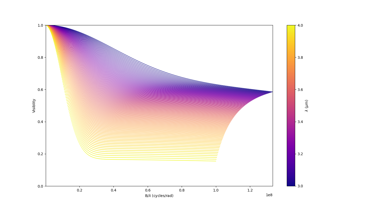
Now that our model is no more circular, we need to take care of the baselines orientations. Let’s plot both North-South and East-West baselines.
fig3v, ax3v = plt.subplots(1, 2, figsize=(14, 5), sharex=True, sharey=True)

# East-West
vis = np.abs(m3.getComplexCoherentFlux(
    spf, spf*0, wls)).reshape(len(wl), len(B))
vis /= np.outer(np.max(vis, axis=1), np.ones(nB))
ax3v[0].scatter(spf, vis, c=wls*1e6, s=0.2, cmap="plasma")
ax3v[0].set_title("East-West Baselines")
ax3v[0].margins(0, 0)
ax3v[0].set_ylim(0, 1)
ax3v[0].set_xlabel("B/$\\lambda$ (cycles/rad)")
ax3v[0].set_ylabel("Visiblity")

# North-South
vis = np.abs(m3.getComplexCoherentFlux(
    spf*0, spf, wls)).reshape(len(wl), len(B))
vis /= np.outer(np.max(vis, axis=1), np.ones(nB))
sc = ax3v[1].scatter(spf, vis, c=wls*1e6, s=0.2, cmap="plasma")
ax3v[1].set_title("North-South Baselines")
ax3v[1].set_xlabel("B/$\\lambda$ (cycles/rad)")
fig3v.colorbar(sc, ax=ax3v.ravel().tolist(), label="$\\lambda$ ($\\mu$m)")
Let’s have a look at our last model’s free parameters.
pprint(m3.getFreeParameters())
... {'c1_eUD_f_interp1': oimParam at 0x23d9e7194f0 : f=2 ± 0  range=[-inf,inf] free=True ,
     'c1_eUD_f_interp2': oimParam at 0x23d9e719520 : f=0.2 ± 0  range=[-inf,inf] free=True ,
     'c1_eUD_elong': oimParam at 0x23d9e7192e0 : elong=2 ± 0  range=[-inf,inf] free=True ,
     'c1_eUD_pa': oimParam at 0x23d9e719490 : pa=90 ± 0 deg range=[-inf,inf] free=True ,
     'c1_eUD_d': oimParam at 0x23d9e7193a0 : d=0.5 ± 0 mas range=[-inf,inf] free=True ,
     'c2_EG_f': oimParam at 0x23d9e7191c0 : f=1 ± 0  range=[-inf,inf] free=True ,
     'c2_EG_elong': oimParam at 0x23d9e7191f0 : elong=2 ± 0  range=[-inf,inf] free=True ,
     'c2_EG_pa': oimParam at 0x23d9e719220 : pa=90 ± 0 deg range=[-inf,inf] free=True ,
     'c2_EG_fwhm_interp1': oimParam at 0x23d9e7192b0 : fwhm=2 ± 0 mas range=[-inf,inf] free=True ,
     'c2_EG_fwhm_interp2': oimParam at 0x23d9e719340 : fwhm=8 ± 0 mas range=[-inf,inf] free=True }
We see here that for the Ellipse (C1_eUD) the f parameter has been replaced by two
independent parameters called c1_eUD_f_interp1 and c1_eUD_f_interp2. They
represent the value of the flux at 3 and 4 microns. We could have added more reference
wavelengths in our model and would have ended with more parameters. The same happens for
the elongated Gaussian (C2_EG) fwhm.
Currently our model has 10 free parameters. In certain cases we might want to link or
share two or more parameters. In our case, we might consider that the two components have
the same pa and elong. This can be done easily. To share a parameter you can just
replace one parameter by another.
eg.params['elong'] = el.params['elong']
eg.params['pa'] = el.params['pa']

pprint(m3.getFreeParameters())
... {'c1_eUD_f_interp1': oimParam at 0x23d9e7194f0 : f=2 ± 0  range=[-inf,inf] free=True ,
     'c1_eUD_f_interp2': oimParam at 0x23d9e719520 : f=0.2 ± 0  range=[-inf,inf] free=True ,
     'c1_eUD_elong': oimParam at 0x23d9e7192e0 : elong=2 ± 0  range=[-inf,inf] free=True ,
     'c1_eUD_pa': oimParam at 0x23d9e719490 : pa=90 ± 0 deg range=[-inf,inf] free=True ,
     'c1_eUD_d': oimParam at 0x23d9e7193a0 : d=0.5 ± 0 mas range=[-inf,inf] free=True ,
     'c2_EG_f': oimParam at 0x23d9e7191c0 : f=1 ± 0  range=[-inf,inf] free=True ,
     'c2_EG_fwhm_interp1': oimParam at 0x23d9e7192b0 : fwhm=2 ± 0 mas range=[-inf,inf] free=True ,
     'c2_EG_fwhm_interp2': oimParam at 0x23d9e719340 : fwhm=8 ± 0 mas range=[-inf,inf] free=True }
That way we have reduced our number of free parameters to 8. If you change the,
for instance, the params['elong'] or el.params['elong'] values it will change
both parameters are they are actually the same instance of the
oimParam class.
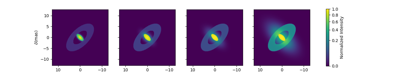
Let’s create a new model which include a elongated ring perpendicular to the Gaussian
and Ellipse pa and with a inner and outer radii equals to 2 and 4 times the ellipse
diameter, respectively.
er = oim.oimERing()
er.params['elong'] = eg.params['elong']
er.params['pa'] = oim.oimParamLinker(eg.params["pa"], "add", 90)
er.params['din'] = oim.oimParamLinker(el.params["d"], "mult", 2)
er.params['dout'] = oim.oimParamLinker(el.params["d"], "mult", 4)

m4 = oim.oimModel([el, eg, er])

fig4im, ax4im, im4 = m4.showModel(256, 0.1, wl=[3e-6, 3.25e-6, 3.5e-6, 4e-6],
                                  figsize=(3.5, 2.5), normPow=0.5, fromFT=fromFT,
                                  normalize=True,
                                  savefig=save_dir / "complexModel_link.png")

Although quite complex this models only have 9 free parameters. If we change the ellipse diameter and its position angle, the components will scale (except the Gaussian that fwhm is independent) and rotate.
el.params['d'].value = 4
el.params['pa'].value = 45

m4.showModel(256, 0.1, wl=[3e-6, 3.25e-6, 3.5e-6, 4e-6], normPow=0.5, figsize=(3.5, 2.5))
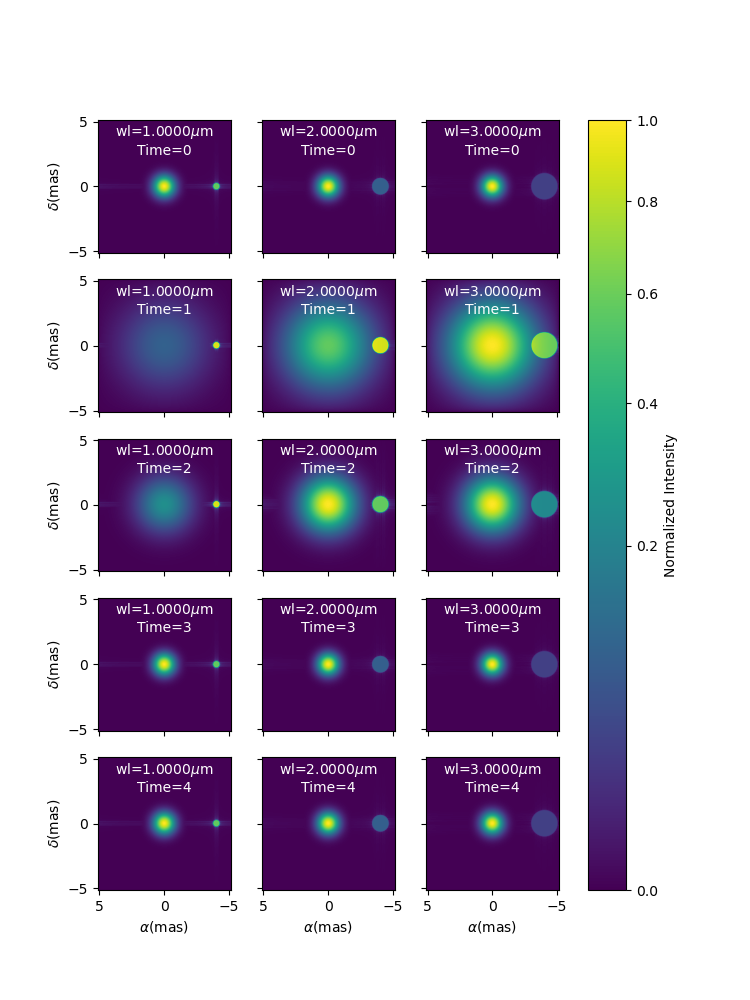
You can also add time dependent parameters to your model using
oimInterpTime <oimodeler.oimParam.oimInterp() class which works similarly to the
oimInterpWl class.
Here, we create a two-components model with a time dependent Gaussian fwhm and a wavelength dependent uniform disk diameter.
gd1 = oim.oimGauss(fwhm=oim.oimInterp('time', mjd=[0, 1, 3], values=[1, 4, 1]))
ud1 = oim.oimUD(d=oim.oimInterp("wl", wl=[1e-6, 3e-6], values=[0.5, 2]), x=-4, y=0, f=0.1)

m5 = oim.oimModel(gd1, ud1)

wls=np.array([1,2,3])*1e-6
times=[0,1,2,3,4]

fig5im, ax5im, im5 = m5.showModel(256, 0.04, wl=wls, t=times, legend=True, figsize=(2.5, 2))
Precomputed chromatic image-cubes
In the FitsImageCubeModels.py.py script, we demonstrate the capability of building models using pre-computed chromatic image-cubes in the fits format.
In this example we will use a chromatic image-cube computed around the \(Br\,\gamma\) emission line for a classical Be Star circumstellar disk. The model, detailed in Meilland et al. (2012) was taken form the AMHRA service of the JMMC.
Note
AMHRA develops and provides various online astrophysical models dedicated to the scientific exploitation of high angular and high spectral facilities. Currently available models are : semi-physical gaseous disk of classical Be stars and dusty disk of YSO, Red-supergiant and AGB, binary spiral for WR stars, physical limb-darkening models, kinematics gaseous disks, and a grid of supergiant B[e] stars models.
Let’s start by importing oimodeler as well as useful packages.
from pathlib import Path
from pprint import pprint

import matplotlib.colors as colors
import matplotlib.cm as cm
import numpy as np
import oimodeler as oim
from matplotlib import pyplot as plt
The fits-formatted image-cube we will use, KinematicsBeDiskModel.fits, is located in the ./examples/AdvancedExamples directory.
path = Path(__file__).parent.parent.parent
file_name = path / "examples" / "AdvancedExamples" / "KinematicsBeDiskModel.fits"
We build our model using a single component of the type
oimComponentFitsImage which
allows to load fits images or image-cubes.
c = oim.oimComponentFitsImage(file_name)
m = oim.oimModel(c)
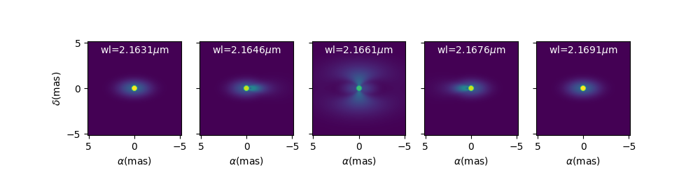
We can now plot images of the model through the \(Br\gamma\) emission line (21661 \(\mu\) m).
wl0, dwl, nwl = 2.1661e-6, 60e-10, 5
wl = np.linspace(wl0-dwl/2, wl0+dwl/2, num=nwl)
m.showModel(256, 0.04, wl=wl, legend=True, normPow=0.4, colorbar=False,
            figsize=(2, 2.5),
            savefig=save_dir / "FitsImageCube_BeDiskKinematicsModel_images.png")
We now compute the visibility for a series of North-South and East-West baselines ranging between 0 and 100m and with the wavelength ranging through the emission line.
nB = 1000
nwl = 51
wl = np.linspace(wl0-dwl/2, wl0+dwl/2, num=nwl)

B = np.linspace(0, 100, num=nB//2)

# 1st half of B array are baseline in the East-West orientation
Bx = np.append(B, B*0)
By = np.append(B*0, B)  # 2nd half are baseline in the North-South orientation

Bx_arr = np.tile(Bx[None, :], (nwl, 1)).flatten()
By_arr = np.tile(By[None, :], (nwl,  1)).flatten()
wl_arr = np.tile(wl[:, None], (1, nB)).flatten()

spfx_arr = Bx_arr/wl_arr
spfy_arr = By_arr/wl_arr

vc = m.getComplexCoherentFlux(spfx_arr, spfy_arr, wl_arr)
v = np.abs(vc.reshape(nwl, nB))
v = v/np.tile(v[:, 0][:, None], (1, nB))
Finally, we plot the results as a function of the wavelength and with a colorscale in terms of the baseline length.
fig, ax = plt.subplots(1, 2, figsize=(8, 4))
titles = ["East-West Baselines", "North-South Baselines"]

for iB in range(nB):
    cB = (iB % (nB//2))/(nB//2-1)
    ax[2*iB//nB].plot(wl*1e9, v[:, iB],
                      color=plt.cm.plasma(cB))

for i in range(2):
    ax[i].set_title(titles[i])
    ax[i].set_xlabel(r"$\lambda$ (nm)")
ax[0].set_ylabel("Visibility")
ax[1].get_yaxis().set_visible(False)

norm = colors.Normalize(vmin=np.min(B), vmax=np.max(B))
sm = cm.ScalarMappable(cmap=plt.cm.plasma, norm=norm)
fig.colorbar(sm, ax=ax, label="B (m)")
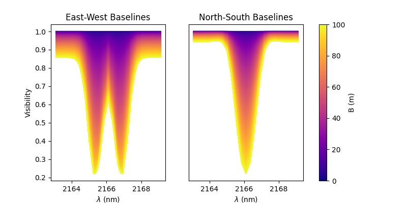
As expected, for a rotating disk (see Meilland et al. (2012) for more details), the visibility for the baselines along the major-axis show a W-shaped profile through the line, whereas the visibliity along the minor-axis of the disk show a V-shaped profile.
Parameters Interpolators
In the previous example, we have introduction parameters interpolators that allow to create chromatic and/or time-dependent models. Here we present in more details these interpolators. This example can be found in the paramInterpolators.py script.
The following table summarize the available interpolators and their parameters. Most of them will be presented in this example.
Class name |
oimInterp macro |
Description |
Parameters |
|---|---|---|---|
oimParamInterpolatorWl |
“wl” |
Interp between key wl |
wl, values |
oimParamInterpolatorTime |
“time” |
Interp between key time |
mjd, values |
oimParamGaussianWl |
“GaussWl” |
Gaussian in wl |
val0, value, x0, fwhm |
oimParamGaussianTime |
“GaussTime” |
Gaussian in time |
val0, value, x0, fwhm |
oimParamMultipleGaussianWl |
“mGaussWl” |
Multiple Gauss. in wl |
val0 and value, x0, fwhm |
oimParamMultipleGaussianTime |
“mGaussTime” |
Multiple Gauss. in time |
val0 and value, x0, fwhm |
oimParamCosineTime |
“cosTime” |
Asym. Cosine in Time |
T0, P, values (optional x0) |
oimParamPolynomialWl |
“polyWl” |
Polynomial in wl |
coeffs |
oimParamPolynomialTime |
“polyTime” |
Polynomial in time |
coeffs |
We start by importing the standard packages.
from pathlib import Path
from pprint import pprint

import matplotlib.pyplot as plt
import matplotlib.colors as colors
import matplotlib.cm as cm
import numpy as np
import oimodeler as oim
In order to simplify plotting the various interpolators we define a plotting function that can works for either a chromatic or a time-dependent model. With some baseline length, wavelength, time vectors passed and some model and interpolated parameter, the function will plot the interpolated parameters as a function of the wavelength or time, and the corresponding visibilities.
def plotParamAndVis(B, wl, t, model, param, ax=None, colorbar=True):
    nB = B.size

    if t is None:
        n = wl.size
        x = wl*1e6
        y = param(wl, 0)
        xlabel = r"$\lambda$ ($\mu$m)"
    else:
        n = t.size
        x = t-60000
        y = param(0, t)
        xlabel = "MJD - 60000 (days)"

    Bx_arr = np.tile(B[None, :], (n, 1)).flatten()
    By_arr = Bx_arr*0

    if t is None:
        t_arr = None
        wl_arr = np.tile(wl[:, None], (1, nB)).flatten()
        spfx_arr = Bx_arr/wl_arr
        spfy_arr = By_arr/wl_arr
    else:
        t_arr = np.tile(t[:, None], (1, nB)).flatten()
        spfx_arr = Bx_arr/wl
        spfy_arr = By_arr/wl
        wl_arr = None

    v = np.abs(model.getComplexCoherentFlux(
        spfx_arr, spfy_arr, wl=wl_arr, t=t_arr).reshape(n, nB))

    if ax is None:
        fig, ax = plt.subplots(2, 1)
    else:
        fig = ax.flatten()[0].get_figure()

    ax[0].plot(x, y, color="r")

    ax[0].set_ylabel("{} (mas)".format(param.name))
    ax[0].get_xaxis().set_visible(False)

    for iB in range(1, nB):
        ax[1].plot(x, v[:, iB]/v[:, 0], color=plt.cm.plasma(iB/(nB-1)))

    ax[1].set_xlabel(xlabel)
    ax[1].set_ylabel("Visibility")

    if colorbar == True:
        norm = colors.Normalize(vmin=np.min(B[1:]), vmax=np.max(B))
        sm = cm.ScalarMappable(cmap=plt.cm.plasma, norm=norm)
        fig.colorbar(sm, ax=ax, label="Baseline Length (m)")

    return fig, ax, v
We will need a baseline length vector (here 200 baselines between 0 and 60m) and we will build for each model either a length 1000 wavelength or time vector.
nB = 200
B = np.linspace(0, 60, num=nB)

nwl = 1000
nt = 1000
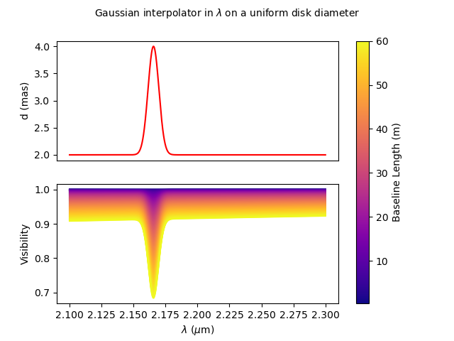
Now, let’s start with our first interpolator: A Gaussian in wavelength (also available for time). It can be used to model spectral features like atomic lines or molecular bands in emission or absorption.
It has 4 parameters :
A central wavelength
x0A value outside the Gaussian (or offset) :
val0A value at the maximum of the Gaussian :
valueA full width at half maximum :
fwhm
To create such an interpolator, we use the class
oimInterp class and specify
GaussWl as the type of interpolator. In our example below we create a Uniform Disk
model with a diameter interpolated between 2 mas (outside the Gaussian range) and 4 mas
at the top of the Gaussian. The central wavelength is set to 2.1656 microns (Brackett
Gamma hydrogen line) and the fwhm to 10nm.
c1 = oim.oimUD(d=oim.oimInterp('GaussWl', val0=2, value=4, x0=2.1656e-6, fwhm=1e-8))
m1 = oim.oimModel(c1)
Finally, we can define the wavelength range and use our custom plotting function.
wl = np.linspace(2.1e-6, 2.3e-6, num=nwl)
fig, ax, im = plotParamAndVis(B, wl, None, m1, c1.params['d'])
fig.suptitle("Gaussian interpolator in $\lambda$ on a uniform disk diameter", fontsize=10)
The parameters of the interpolator can be accessed using the params attribute of the
oimParamInterpolator:
pprint(c1.params['d'].params)
... [oimParam at 0x2610e25e220 : x0=2.1656e-06 ± 0 m range=[0,inf] free=True ,
     oimParam at 0x2610e25e250 : fwhm=1e-08 ± 0 m range=[0,inf] free=True ,
     oimParam at 0x2610e25e280 : d=2 ± 0 mas range=[-inf,inf] free=True ,
     oimParam at 0x2610e25e2b0 : d=4 ± 0 mas range=[-inf,inf] free=True ]
Each one can also be accessed using their name as an attribute:
pprint(c1.params['d'].x0)
... oimParam x0 = 2.1656e-06 ± 0 m range=[0,inf] free
These parameters will behave like normal free or fixed parameters when performing model
fitting. We can get the full list of parameters from our model using the
getParameter method.
pprint(m1.getParameters())
... {'c1_UD_x': oimParam at 0x2610e25e100 : x=0 ± 0 mas range=[-inf,inf] free=False ,
     'c1_UD_y': oimParam at 0x2610e25e130 : y=0 ± 0 mas range=[-inf,inf] free=False ,
     'c1_UD_f': oimParam at 0x2610e25e160 : f=1 ± 0  range=[-inf,inf] free=True ,
     'c1_UD_d_interp1': oimParam at 0x2610e25e220 : x0=2.1656e-06 ± 0 m range=[0,inf] free=True ,
     'c1_UD_d_interp2': oimParam at 0x2610e25e250 : fwhm=1e-08 ± 0 m range=[0,inf] free=True ,
     'c1_UD_d_interp3': oimParam at 0x2610e25e280 : d=2 ± 0 mas range=[-inf,inf] free=True ,
     'c1_UD_d_interp4': oimParam at 0x2610e25e2b0 : d=4 ± 0 mas range=[-inf,inf] free=True }
In the dictionary returned by the getParameters method, the four interpolator parameters
are called c1_UD_d_interpX.
The second interpolator presented here is the multiple Gaussian in wavelength (also
available for time). It is a generalisation of the first interpolator but with
multiple values for x0, fwhm and values.
c2 = oim.oimUD(f=0.5, d=oim.oimInterp("mGaussWl", val0=2, values=[4, 0, 0],
                                      x0=[2.05e-6, 2.1656e-6, 2.3e-6],
                                      fwhm=[2e-8, 2e-8, 1e-7]))
pt = oim.oimPt(f=0.5)
m2 = oim.oimModel(c2, pt)

c2.params['d'].values[1] = oim.oimParamLinker(
    c2.params['d'].values[0], "mult", 3)
c2.params['d'].values[2] = oim.oimParamLinker(
    c2.params['d'].values[0], "add", -1)

wl = np.linspace(1.9e-6, 2.4e-6, num=nwl)

fig, ax, im = plotParamAndVis(B, wl, None, m2, c2.params['d'])
fig.suptitle(
    "Multiple Gaussian interpolator in $\lambda$ on a uniform disk diameter", fontsize=10)
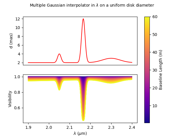
Here, to reduce the number of free parameters of the model with have linked the second
and third values of the interpolator to the first one.
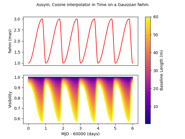
Let’s look at our third interpolator: An asymmetric cosine interpolator in time. As it is cyclic it might be used to simulated a cyclic variation, for example a pulsating star.
It has 5 parameters :
The Epoch (mjd) of the minimum value:
T0.The period of the variation in days
P.The mini and maximum values of the parameter as a two-elements array :
value.Optionally, the asymmetry :
x0(x0=0.5 means no assymetry, x0=0 or 1 maximum asymmetry).
c3 = oim.oimGauss(fwhm=oim.oimInterp(
    "cosTime", T0=60000, P=1, values=[1, 3], x0=0.8))
m3 = oim.oimModel(c3)

t = np.linspace(60000, 60006, num=nt)
wl = 2.2e-6

fig, ax, im = plotParamAndVis(B, wl, t, m3, c3.params['fwhm'])
fig.suptitle(
    "Assym. Cosine interpolator in Time on a Gaussian fwhm", fontsize=10)
Now, let’s have a look at the classic wavelength interpolator (also available for time). jIt has two parameters:
A list of reference wavelengths:
wl.A list of values at the reference wavelengths:
values.
Values will be interpolated in the range, using either linear (default), quadratic, or
cubic interpolation set by the keyword kind. Outside the range of defined wavelengths
the values will be either fixed (default) or extrapolated depending on the value of the
extrapolate keyword.
Here, we present examples with the three kind of interpolation and with or without extrapolation.
c4 = oim.oimIRing(d=oim.oimInterp("wl", wl=[2e-6, 2.4e-6, 2.7e-6, 3e-6], values=[2, 6, 5, 6],
                                  kind="linear", extrapolate=True))
m4 = oim.oimModel(c4)
wl = np.linspace(1.8e-6, 3.2e-6, num=nwl)
fig, ax = plt.subplots(2, 6, figsize=(18, 6), sharex=True, sharey="row")

plotParamAndVis(B, wl, None, m4, c4.params['d'], ax=ax[:, 0], colorbar=False)
c4.params['d'].extrapolate = False
plotParamAndVis(B, wl, None, m4, c4.params['d'], ax=ax[:, 1], colorbar=False)

c4.params['d'].extrapolate = True
c4.params['d'].kind = "quadratic"
plotParamAndVis(B, wl, None, m4, c4.params['d'], ax=ax[:, 2], colorbar=False)
c4.params['d'].extrapolate = False
plotParamAndVis(B, wl, None, m4, c4.params['d'], ax=ax[:, 3], colorbar=False)

c4.params['d'].extrapolate = True
c4.params['d'].kind = "cubic"
plotParamAndVis(B, wl, None, m4, c4.params['d'], ax=ax[:, 4], colorbar=False)
c4.params['d'].extrapolate = False
plotParamAndVis(B, wl, None, m4, c4.params['d'], ax=ax[:, 5], colorbar=False)

plt.subplots_adjust(left=0.05, bottom=0.1, right=0.99, top=0.9,
                    wspace=0.05, hspace=0.05)
for i in range(1, 6):
    ax[0, i].get_yaxis().set_visible(False)
    ax[1, i].get_yaxis().set_visible(False)

fig.suptitle("Linear, Quadratic and Cubic interpolators (with extrapolation"
             r" or fixed values outside the range) in $\lambda$ on a uniform"
             " disk diameter", fontsize=18)

Finally, we can also use a polynominal interpolator in time (also available for
wavelength). Its free parameters are the coefficients of the polynomial. The parameter
x0 allows to shift the reference time (in mjd) from 0 to an arbitrary date.
c5 = oim.oimUD(d=oim.oimInterp('polyTime', coeffs=[1, 3.5, -0.5], x0=60000))
m5 = oim.oimModel(c5)

wl = 2.2e-6
t = np.linspace(60000, 60006, num=nt)

fig, ax, im = plotParamAndVis(B, wl, t, m5, c5.params['d'])
fig.suptitle(
    "Polynomial interpolator in Time on a uniform disk diameter", fontsize=10)

As for other part of the oimodeler software, oimParamInterpolator was designed so that users can easily create their own interoplators using inheritage. See the Creating New Interpolators example.
Fitting a chromatic model
In the example chromaticModelFit.py we will show how to perform model-fitting with a simple chromatic model.
We will use some ASPRO-simulated data that were computed using a chromatic image-cubes
exported from the same oimodeler model used for model fitting.
Let’s first start by importing packages and setting the path to the data directory.
from pathlib import Path
from pprint import pprint

import numpy as np
import oimodeler as oim


path = Path(__file__).parent.parent.parent
data_dir = path / "examples" / "testData" / "ASPRO_CHROMATIC_SKWDISK"
save_dir = path / "images"
product_dir = path / "examples" / "testData" / "IMAGES"
if not save_dir.exists():
    save_dir.mkdir(parents=True)
if not product_dir.exists():
    product_dir.mkdir(parents=True)
We will build a model mimicing a star (uniform disk) and the inner rim of a dusty disk (Skewed ring). The flux ratio between the two components will depend on the wavelength as well as the outer radius of the skewed ring.
star = oim.oimUD(d=1, f=oim.oimInterp(
    "wl", wl=[3e-6, 4e-6], values=[0.5, 0.1]))
ring = oim.oimESKRing(din=8, dout=oim.oimInterp(
    "wl", wl=[3e-6, 4e-6], values=[9, 14]), elong=1.5, skw=0.8, pa=50)
ring.params['f'] = oim.oimParamNorm(star.params['f'])
ring.params["skwPa"] = oim.oimParamLinker(ring.params["pa"], "add", 90)
model = oim.oimModel(star, ring)
We used the oimInterp class with the "wl" option
to build a linear interpolator for the parameter f of the uniform disk with two
reference wavlengths at 3 and 4 microns with a value of the flux of 0.5 and 0.1,
respectively. We also link the flux of the skewed ring so that the total flux is
normalized. The ring outer radius dout is also interpolated between 9 mas at
3 microns and 14 at 4 microns. Finally, we set the ring skweness position angle
skwPa to be perpendicular to the ring major-axis (set with the pa parameter).
We can have a look at our model at three wavelengths 3, 3.5 and 4 microns.
model.showModel(256, 0.06, wl=np.linspace(3., 4, num=3)*1e-6, legend=True,
                normalize=True, normPow=1, fromFT=True,
                savefig=save_dir / "chromaticModelFitImageInit.png")

The simulated data that we will use where created with fits-formated image-cube
computed with this image using the getImage method with the toFits=True option.
Here we simulate 50 wavelengths for the cube as ASPRO doesn’t interpolate between
wavelengths of imported image-cube yet.
img = model.getImage(256, 0.06, toFits=True, fromFT=True,
                     wl=np.linspace(3, 4, num=50)*1e-6)
img.writeto(product_dir / "skwDisk.fits", overwrite=True)
Using this model and the ASPRO software, we have simulated 3 MATISSE observations: One with each of the available standard configuration of the ATs telescopes at VLTI: small, medium and large. The three observations were exported as a single OIFITS file.
Let’s load it into a oimData object, and apply an
filter from the oimDataFilter module that will keep
only VISDATA2 and T3PHI more the model-fitting process.
files = list(map(str, data_dir.glob("*.fits")))
data = oim.oimData(files)
f1 = oim.oimRemoveArrayFilter(targets="all", arr=["OI_VIS", "OI_FLUX"])
f2 = oim.oimDataTypeFilter(targets="all", dataType=["T3AMP"])
data.setFilter(oim.oimDataFilter([f1, f2]))
Let’s have a look at our model’s free parameters:
params = model.getFreeParameters()
pprint(params)
... {'c1_UD_d': oimParam at 0x2a0edc241c0 : d=1 ± 0 mas range=[-inf,inf] free=True ,
     'c1_UD_f_interp1': oimParam at 0x2a0edc242b0 : f=0.5 ± 0  range=[-inf,inf] free=True ,
     'c1_UD_f_interp2': oimParam at 0x2a0edc242e0 : f=0.1 ± 0  range=[-inf,inf] free=True ,
     'c2_SKER_din': oimParam at 0x2a0edc24220 : din=8 ± 0 mas range=[-inf,inf] free=True ,
     'c2_SKER_dout_interp1': oimParam at 0x2a0edc24e80 : dout=9 ± 0 mas range=[-inf,inf] free=True ,
     'c2_SKER_dout_interp2': oimParam at 0x2a0edc24e50 : dout=14 ± 0 mas range=[-inf,inf] free=True ,
     'c2_SKER_elong': oimParam at 0x2a0edc24310 : elong=1.5 ± 0  range=[-inf,inf] free=True ,
     'c2_SKER_pa': oimParam at 0x2a0edc24400 : pa=50 ± 0 deg range=[-inf,inf] free=True ,
     'c2_SKER_skw': oimParam at 0x2a0edc24460 : skw=0.8 ± 0  range=[-inf,inf] free=True }
Here, we see that the flux of the uniform disk and the outer radius of the skewed ring
have both been replaced by two parameters representing thir respective values at the
reference wavelengths: c1_UD_f_interp1 is the flux at 3 microns and
c1_UD_f_interp2 the flux at 4 microns.
Before running the fit we need to set the parameter space for all free parameters:
params['c1_UD_f_interp1'].set(min=0.0, max=1)
params['c1_UD_f_interp2'].set(min=-0.0, max=1)
params['c1_UD_d'].set(min=0, max=5, free=True)
params['c2_SKER_pa'].set(min=0., max=180)
params['c2_SKER_elong'].set(min=1, max=3)
params['c2_SKER_din'].set(min=5, max=20.)
params['c2_SKER_skw'].set(min=0, max=1.5)
params['c2_SKER_dout_interp1'].set(min=5., max=30.)
params['c2_SKER_dout_interp2'].set(min=5., max=30.)
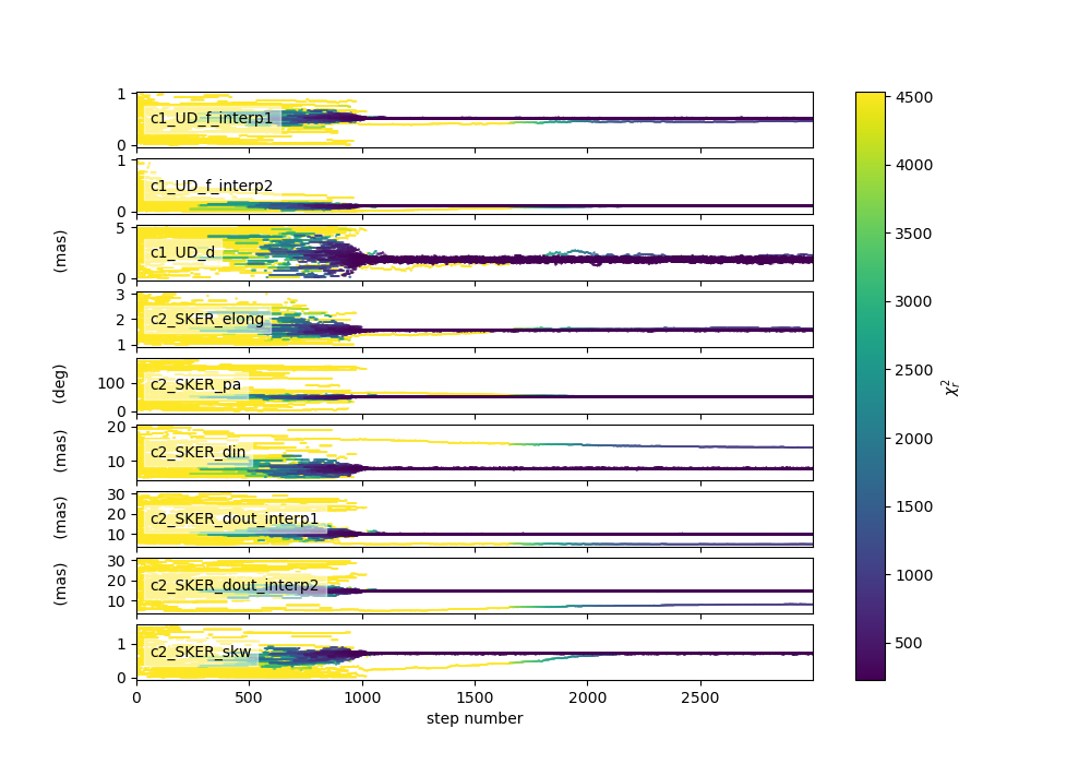
Now we can perform the model-fitting using the emcee <https://emcee.readthedocs.io/en/stable/> -based fitter with 30 walkers, 2000 steps and starting at a random position within the parameter space.
fit = oim.oimFitterEmcee(data, model, nwalkers=50)
fit.prepare(init="random")
fit.run(nsteps=3000, progress=True)
Plotting the walkers and the corner plot (discarding the first half of the steps of the run).
figWalkers, axeWalkers = fit.walkersPlot()
figCorner, axeCorner = fit.cornerPlot(discard=1000)
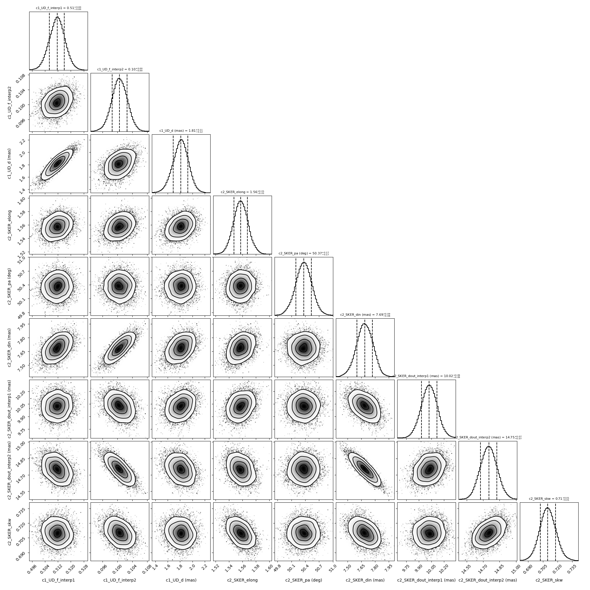
Finally, getting the best parameters and the uncertainties and plotting the fit data.
median, err_l, err_u, err = fit.getResults(mode='best', discard=1000)
fit.simulator.plot(["VIS2DATA", "T3PHI"])
