Expanding the Software
In this section we present examples that show how to expand the functionality
of the oimodeler software by creating customs objects:
oimComponents,
oimFilters,
oimFitters, and custom plotting
functions or utils.
Creating New Components
Box (Fourier plan formula)
In the createCustomComponentFourier.py
example we show how to implement a new model component using a formula in the Fourier plane.
The component will inherit from the oimComponentFourier
class. The Fourier formula should be implemented as the
oimComponentFourier._visFunction
method and, optionally, the formula in the image plan can be implemented using the
oimComponentFourier._imageFunction
method.
For this example we will show how to implement a basic rectangular box component. We start by importing the required packages:
from pathlib import Path

import astropy.units as u
import matplotlib.pyplot as plt
import numpy as np
import oimodeler as oim
Our new component will be named oimBox, and it will have two parameters,
dx and dy the size of the box in the x and y directions. Let’s start to
implement the oimBox class and its __init__ method.
class oimBox(oim.oimComponentFourier):
    name = "2D Box"
    shortname = "BOX"

    def __init__(self, **kwargs):
        super().__init__(**kwargs)
        self.params["dx"] = oim.oimParam(
            name="dx", value=1, description="Size in x", unit=u.mas)
        self.params["dy"] = oim.oimParam(
            name="dy", value=1, description="Size in y", unit=u.mas)
        self._eval(**kwargs)
The class inherits from oimComponentFourier.
The __init__ method is called with the **kwargs to allow the passing of keyword
arguments. To inherit from the parent class, we first call its
initialization method with super().__init__. Then, we define the two new parameters,
dx and dy, which are instances of the
oimParam class. Finally, we need to call the
oimComponent._eval method that allows
the parameters to be processed.
Now that the new class is created, we need to implement its
oimComponent._visFunction method,
with the Fourier transform formula of our component. This method is called when using
the oimComponent.getComplexCoherentFlux
method.
Note that the component parameters should be called with (wl, t), to allow parameter chromaticity and time dependence. The parameters have a unit. This unit should also be used to allow the use of other units (via unit conversion) when creating instances of the component.
In our case, the complex visibilty of a rectangle is quite easy to write. It is a simple 2D-sinc function. Note that the x and y sizes are converted from the given unit (usually mas) to rad.
def _visFunction(self, ucoord, vcoord, rho, wl, t):
    x = self.params["dx"](wl, t)*self.params["dx"].unit.to(u.rad)*ucoord
    y = self.params["dy"](wl, t)*self.params["dy"].unit.to(u.rad)*vcoord
    return np.sinc(x)*np.sinc(y)
We also need to implement the image that will be created when using the
oimComponent.getImage method.
If not implemented, the model will use the Fourier based formula to compute the image.
It will also be the case if the keyword fromFT is set to True, when calling
the getImage method.
However, it is always interesting to implement the image method, at least for
debugging purposes, to check that the image computed with the image formula and
using the fromFT option gives compatible results. We will see that a bit later
in an example.
For our box, we can implement the image method with logical operations
def _imageFunction(self, xx, yy, wl, t):
    return ((np.abs(xx) <= self.params["dx"](wl, t)/2) &
            (np.abs(yy) <= self.params["dy"](wl, t)/2)).astype(float)
The full code of the oimBox component is quite short.
class oimBox(oim.oimComponentFourier):
    name = "2D Box"
    shortname = "BOX"

    def __init__(self, **kwargs):
        super().__init__(**kwargs)
        self.params["dx"] = oim.oimParam(
            name="dx", value=1, description="Size in x", unit=u.mas)
        self.params["dy"] = oim.oimParam(
            name="dy", value=1, description="Size in y", unit=u.mas)
        self._eval(**kwargs)

    def _visFunction(self, ucoord, vcoord, rho, wl, t):
        x = self.params["dx"](wl, t)*self.params["dx"].unit.to(u.rad)*ucoord
        y = self.params["dy"](wl, t)*self.params["dy"].unit.to(u.rad)*vcoord
        return np.sinc(x)*np.sinc(y)

    def _imageFunction(self, xx, yy, wl, t):
        return ((np.abs(xx) <= self.params["dx"](wl, t)/2) &
                (np.abs(yy) <= self.params["dy"](wl, t)/2)).astype(float)
We can now use it as we do with any other oimodeler component. Let’s build our first
model with it.
b1 = oimBox(dx=40, dy=10)
m1 = oim.oimModel([b1])
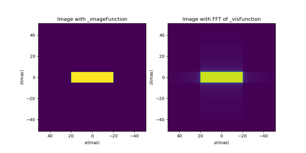
Now we can create images of our model:
In the image plane with the
_imageFunction.In the Fourier plane with the
_visFunction(with the FFT).
Both can be plotted with the oimModel.showModel
method. To create the image from the FFT of the visibilty function, we just need to set
the fromFT keyword to True.
fig, ax = plt.subplots(1, 2, figsize=(10,5))
m1.showModel(512, 0.2, axe=ax[0], colorbar=False)
m1.showModel(512, 0.2, axe=ax[1], fromFT=True, colorbar=False)
ax[0].set_title("Image with _imageFunction")
ax[1].set_title("Image with FFT of _visFunction")
Of course, as our oimBox inherits from the
oimComponent class,
it has three addtional parameters available: Its position described by x and y,
and the flux f. All components can also be rotated using the position angle pa
parameter. Note, that if elliptic=True is not set at the component creation
as a class variable, the postion angle pa parameters (and the elong parameter)
are not added to the model.
Let’s create a complex model with boxes and uniform disk.
b2 = oimBox(dx=2, dy=2, x=-20, y=0, f=0.5)
b3 = oimBox(dx=10, dy=20, x=30, y=10, pa=-40, f=10)
c = oim.oimUD(d=10, x=30, y=10)
m2 = oim.oimModel([b1, b2, b3, c])
m2.showModel(512, 0.2, colorbar=False, figsize=(5, 5))

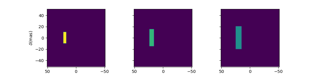
We could also create a chromatic box component using the
oimInterpWl class or link parameters with
the oimParamLinker class.
b4 = oimBox(dx=oim.oimInterpWl([2e-6, 2.4e-6], [5, 10]), dy=2, x=20, y=0, f=0.5)
b4.params['dy'] = oim.oimParamLinker(b4.params['dx'], 'mult', 4)

m3 = oim.oimModel([b4])
m3.showModel(512, 0.2, wl=[2e-6, 2.2e-6, 2.4e-6], colorbar=False, swapAxes=True)
Let’s finish this example by plotting the visibility of such models for a set of East-West and North-South baselines and wavelengths in the K-band.
nB = 200  # number of baselines
nwl = 50  # number of walvengths

# Create some spatial frequencies
wl = np.linspace(2e-6, 2.5e-6, num=nwl)
B = np.linspace(1, 100, num=nB)
Bs = np.tile(B, (nwl, 1)).flatten()
wls = np.transpose(np.tile(wl, (nB, 1))).flatten()
spf = Bs/wls
spf0 = spf*0

fig, ax=plt.subplots(3, 2, figsize=(10, 7))

models=[m1, m2, m3]
names =["1 Box", "Multi Boxes","Chromatic box"]

for i, m in enumerate(models):
    visWest = np.abs(m.getComplexCoherentFlux(spf, spf0, wls)).reshape(nwl, nB)
    visWest /= np.outer(np.max(visWest, axis=1), np.ones(nB))
    visNorth = np.abs(m.getComplexCoherentFlux(
        spf0, spf, wls)).reshape(nwl, nB)
    visNorth /= np.outer(np.max(visNorth, axis=1), np.ones(nB))

    cb = ax[i, 0].scatter(spf, visWest, c=wls*1e6, s=0.2, cmap="plasma")
    ax[i, 1].scatter(spf, visNorth, c=wls*1e6, s=0.2, cmap="plasma")
    ax[i, 0].set_ylabel(f"Vis. of {names[i]}")

    if i != 2:
        ax[i, 0].get_xaxis().set_visible(False)
        ax[i, 1].get_xaxis().set_visible(False)

    ax[i, 1].get_yaxis().set_visible(False)

ax[2,0].set_xlabel("B/$\\lambda$ (cycles/rad)")
ax[2,1].set_xlabel("B/$\\lambda$ (cycles/rad)")
ax[0,0].set_title("East-West baselines")
ax[0,1].set_title("North-South baselines")
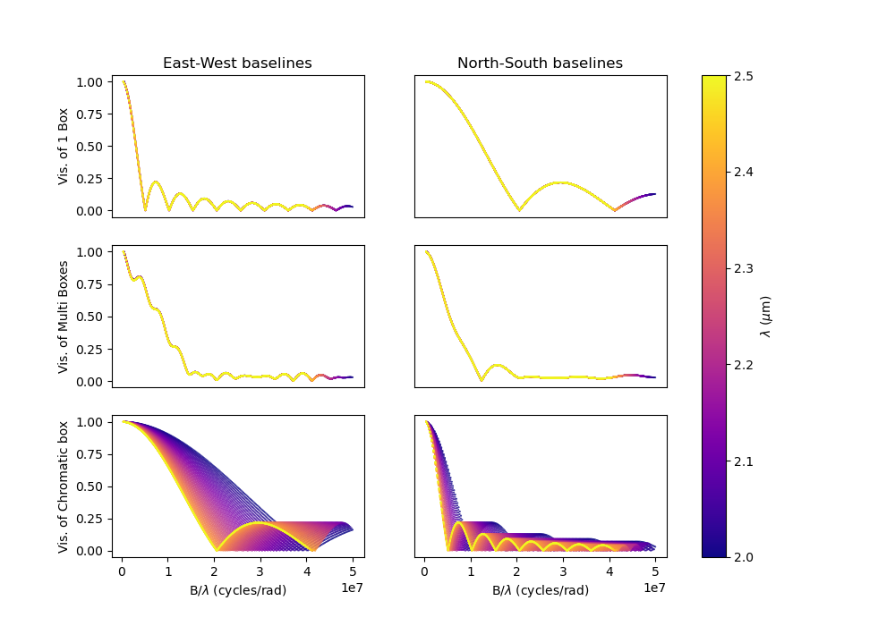
Of course, only the third model is chromatic.
Fast Rotator (External model)
In the createCustomComponentImageFastRotator.py
example, we will create a new component derived from the
oimImageComponent, using an
external function that return a chromatic image cube.
The model is a simple implementation of a fast rotating star flattened by rotation (Roche Model) including gravity darkening (\(T_{eff}\propto g_{eff}^\beta\)). The emission is a simple blackbody.
First, let’s import a few packages used in this example:
from pathlib import Path

import matplotlib.colors as colors
import matplotlib.cm as cm
import matplotlib.pyplot as plt
import numpy as np
import oimodeler as oim
from astropy import units as units
Here is the code of the fastRotator external function that we want to
encapsulate into a oimComponent
to be used in oimodeler.
def fastRotator(dim0, size, incl, rot, Tpole, lam, beta=0.25):
    h = 6.63e-34
    c = 3e8
    kb = 1.38e-23

    a = 2./3*(rot)**0.4+1e-9
    K = np.sin(1./3.)*np.pi

    K1 = h*c/kb
    nlam = np.size(lam)
    incl = np.deg2rad(incl)

    x0 = np.linspace(-size, size, num=dim0)
    idx = np.where(np.abs(x0) <= 1.5)
    x = np.take(x0, idx)
    dim = np.size(x)
    unit = np.ones(dim)
    x = np.outer(x, unit)
    x = np.einsum('ij, k->ijk', x, unit)

    y = np.swapaxes(x, 0, 1)
    z = np.swapaxes(x, 0, 2)

    yp = y*np.cos(incl)+z*np.sin(incl)
    zp = y*np.sin(incl)-z*np.cos(incl)

    r = np.sqrt(x**2+yp**2+zp**2)
    theta = np.arccos(zp/r)

    x0 = (1.5*a)**1.5*np.sin(1e-99)
    r0 = a*np.sin(1/3.)*np.arcsin(x0)/(1.0/3.*x0)

    x2 = (1.5*a)**1.5*np.sin(theta)
    rin = a*np.sin(1/3.)*np.arcsin(x2)/(1.0/3.*x2)

    rhoin = rin*np.sin(theta)/a/K
    dr = (rin/r0-r) >= 0
    Teff = Tpole*(np.abs(1-rhoin*a)**beta)

    if nlam == 1:
        flx = 1./(np.exp(K1/(lam*Teff))-1)

        im = np.zeros([dim, dim])

        for iz in range(dim):
            im = im*(im != 0)+(im == 0) * \
                dr[:, :, iz]*flx[:, :, iz]  # *limb[:,:,iz]

        im = np.rot90(im)

        tot = np.sum(im)
        im = im/tot
        im0 = np.zeros([dim0, dim0])

        im0[dim0//2-dim//2:dim0//2+dim//2, dim0//2-dim//2:dim0//2+dim//2] = im
    else:
        unit = np.zeros(nlam)+1
        dr = np.einsum('ijk, l->ijkl', dr, unit)
        flx = 1./(np.exp(K1/np.einsum('ijk, l->ijkl', Teff, lam))-1)
        im = np.zeros([dim, dim, nlam])

        for iz in range(dim):
            im = im*(im != 0)+dr[:, :, iz, :]*flx[:, :, iz, :]*(im == 0)

        im = np.rot90(im)
        tot = np.sum(im, axis=(0, 1))
        for ilam in range(nlam):
            im[:, :, ilam] = im[:, :, ilam]/tot[ilam]

        im0 = np.zeros([dim0, dim0, nlam])
        im0[dim0//2-dim//2:dim0//2+dim//2, dim0//2-dim//2:dim0//2+dim//2, :] = im
        return im0
Now, we will define the new class for the fast rotator model. It will be derived
from the oimComponentImage class
as the model is defined in the image plane. We first write the __init__ method
of the new class. It needs to includes all the model parameters.
class oimFastRotator(oim.oimComponentImage):
    name = "Fast Rotator"
    shortname = "FRot"

    def __init__(self, **kwargs):
        super(). __init__(**kwargs)

        self.params["incl"] = oim.oimParam(
            name="incl", value=0, description="Inclination angle", unit=units.deg)
        self.params["rot"] = oim.oimParam(
            name="rot", value=0, description="Rotation Rate", unit=units.one)
        self.params["Tpole"] = oim.oimParam(
            name="Tpole", value=20000, description="Polar Temperature", unit=units.K)
        self.params["dpole"] = oim.oimParam(
            name="dplot", value=1, description="Polar diameter", unit=units.mas)
        self.params["beta"] = oim.oimParam(
            name="beta", value=0.25, description="Gravity Darkening Exponent", unit=units.one)

        self._t = np.array([0])
        self._wl = np.linspace(0.5e-6, 15e-6, num=10)
        self._eval(**kwargs)
Note
Unlike for models defined in the Fourier plane, you need to define the internal
wavelength self._wl and time self._t grids with their respective class
attributes.
Here, we set the time to a fixed value so that the model will be time independent. The wavelength dependence of the model is set to a vector of 10 reference wavelengths between 0.5 and 15 microns. This will be used to compute reference images and linear interpolation in wavelength will be used on the Fourier transforms of the images.
Together with the parameter dim (dimension of the image in x and y), the self._wl
and the self._t set the length dimensions of the internal image hypercube
(4-dimensional: x, y, wl, and t).
Now we can implement the call to the fastRotator function. As it is an external
function that computes its own spatial and spectral grid we need to implement
it in the oimComponentImage._internalImage
method.
def _internalImage(self):
    dim = self.params["dim"].value
    incl = self.params["incl"].value
    rot = self.params["rot"].value
    Tpole = self.params["Tpole"].value
    dpole = self.params["dpole"].value
    beta = self.params["beta"].value

    im = fastRotator(dim, 1.5, incl, rot, Tpole, self._wl, beta=beta)
    im = np.tile(np.moveaxis(im, -1, 0)[None, :, :, :], (1, 1, 1, 1))
    self._pixSize = 1.5*dpole/dim*units.mas.to(units.rad)
    return im
Here we need to reshape the result of the fastRotator function to the proper
shape for an internal image of the oimImageComponent
class. The FastRotator returns a 3D image-cube (x, y, wl). We move its axis and
reshape it to a 4D image-hypercube (t, wl, x, y).
Finally, we need to set the pixel size (in rad) using the self._pixSize
private attribute. For our example, we compute a fastRotator on a grid of
1.5 polar diameter (because the equatorial diameter goes up to 1.5 polar diameter
for a critically rotating star). The pixel size formula depends on the dpole and
dim parameters.
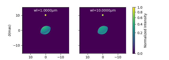
Let’s build our first model with this brand new component.
c = oimFastRotator(dpole=5, dim=128, incl=-70, rot=0.99, Tpole=20000, beta=0.25)
m = oim.oimModel(c)
We can now plot the model images at various wavelengths as we do for any other
oimModel.
m.showModel(512, 0.025, wl=[1e-6, 10e-6 ], legend=True, normalize=True)

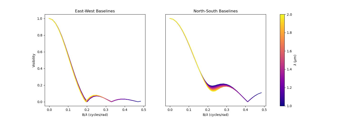
Let’s create a some spatial frequencies, with some chromaticity. For that we create baselines in the East-West and North-South orientations.
nB = 1000
nwl = 20
wl = np.linspace(1e-6, 2e-6, num=nwl)

B = np.linspace(0, 100, num=nB//2)

# 1st half of B array are baseline in the East-West orientation
Bx = np.append(B, B*0)
By = np.append(B*0, B)  # 2nd half are baseline in the North-South orientation

Bx_arr = np.tile(Bx[None, :], (nwl, 1)).flatten()
By_arr = np.tile(By[None, :], (nwl,  1)).flatten()
wl_arr = np.tile(wl[:, None], (1, nB)).flatten()

spfx_arr = Bx_arr/wl_arr
spfy_arr = By_arr/wl_arr
We now compute the complex coherent flux and then extract the visiblity from it. Note that the model is already normalized to one so that we don’t need to divide the complex coherent flux by the zero frequency.
vc = m.getComplexCoherentFlux(spfx_arr, spfy_arr, wl_arr)
v = np.abs(vc.reshape(nwl, nB))
Finally, we plot the East-West and North-South visiblity with a colorscale for the wavelength.
fig, ax = plt.subplots(1, 2, figsize=(15, 5))
titles = ["East-West Baselines", "North-South Baselines"]
for iwl in range(nwl):
    cwl = iwl/(nwl-1)
    ax[0].plot(B/wl[iwl]/units.rad.to(units.mas), v[iwl, :nB//2],
               color=plt.cm.plasma(cwl))
    ax[1].plot(B/wl[iwl]/units.rad.to(units.mas), v[iwl, nB//2:],
               color=plt.cm.plasma(cwl))

for i in range(2):
    ax[i].set_title(titles[i])
    ax[i].set_xlabel("B/$\lambda$ (cycles/rad)")
ax[0].set_ylabel("Visibility")
ax[1].get_yaxis().set_visible(False)

norm = colors.Normalize(vmin=np.min(wl)*1e6, vmax=np.max(wl)*1e6)
sm = cm.ScalarMappable(cmap=plt.cm.plasma, norm=norm)
fig.colorbar(sm, ax=ax, label="$\\lambda$ ($\\mu$m)")
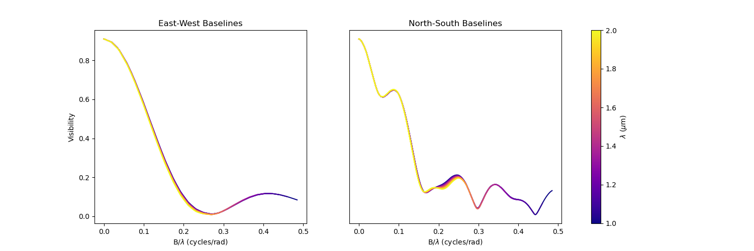
This new oimfastRotator component can be rotated and used together with other
oimComponent classes to build more
complex models.
Here, we add a uniform disk component
oimUD:
c.params['f'].value = 0.9
c.params['pa'].value = 30
ud = oim.oimUD(d=1, f=0.1, y=10)
m2 = oim.oimModel(c, ud)
And finally, we produce the same plots as before for this new complex model.
m2.showModel(512, 0.06, wl=[1e-6, 10e-6], legend=True, normalize=True, normPow=0.5,
             savefig=save_dir / "customCompImageFastRotator2.png")
vc = m2.getComplexCoherentFlux(spfx_arr, spfy_arr, wl_arr)
v = np.abs(vc.reshape(nwl, nB))

fig, ax = plt.subplots(1, 2, figsize=(15, 5))
titles = ["East-West Baselines", "North-South Baselines"]
for iwl in range(nwl):
    cwl = iwl/(nwl-1)
    ax[0].plot(B/wl[iwl]/units.rad.to(units.mas), v[iwl, :nB//2],
               color=plt.cm.plasma(cwl))
    ax[1].plot(B/wl[iwl]/units.rad.to(units.mas), v[iwl, nB//2:],
               color=plt.cm.plasma(cwl))

for i in range(2):
    ax[i].set_title(titles[i])
    ax[i].set_xlabel("B/$\lambda$ (cycles/rad)")
ax[0].set_ylabel("Visibility")
ax[1].get_yaxis().set_visible(False)

norm = colors.Normalize(vmin=np.min(wl)*1e6, vmax=np.max(wl)*1e6)
sm = cm.ScalarMappable(cmap=plt.cm.plasma, norm=norm)
fig.colorbar(sm, ax=ax, label="$\\lambda$ ($\\mu$m)")
Spiral (Image plan formula)
In the createCustomComponentImageSpiral.py
example we will create a new component derived from the
oimImageComponent class,
which describes a logarithmic spiral.
But first let’s import a few packages used in this example:
from pathlib import Path

import matplotlib.pyplot as plt
import numpy as np
import oimodeler as oim
from astropy import units as units
Now we will define the new class for the spiral model. Again, it will be derived from
the oimComponentImage class as the model is defined
in the image plane. We first write the __init__ method of the new class.
It needs to includes all the model’s parameters.
class oimSpiral(oim.oimComponentImage):
    name = "Spiral component"
    shorname = "Sp"
    elliptic = True

    def __init__(self, **kwargs):
        super(). __init__(**kwargs)
        self.params["fwhm"] = oim.oimParam(**oim._standardParameters["fwhm"])
        self.params["P"] = oim.oimParam(name="P",
                                        value=1, description="Period in mas", unit=units.mas)
        self.params["width"] = oim.oimParam(name="width",
                                            value=0.01, description="Width as filling factor", unit=units.one)

        self._pixSize = 0.05*units.mas.to(units.rad)
        self._t = np.array([0])  # constant value <=> static model
        self._wl = np.array([0])  # constant value <=> achromatic model
        self._eval(**kwargs)
Here we chose to fix the pixel size in the __init__ method. As we don’t
intend to have chromaticity, we fixed the internal time and wavelength arrays.
Unlike in the previous example, as we don’t use an externally computed image,
so we can implement the oimComponentImage._imageFunction
of the class instead of the
oimComponentImage._internaImage
one.
The main difference is that the
oimComponentImage._imageFunction
directly provides the 4D-grid in time, wavelength and x and y.
def _imageFunction(self, xx, yy, wl, t):
    # As xx and yy are transformed coordinates, r and phi takes into account
    # the ellipticity and orientation using the pa and elong keywords
    r = np.sqrt(xx**2+yy**2)
    phi = np.arctan2(yy, xx)

    p = self.params["P"](wl, t)
    sig = self.params["fwhm"](wl, t)/2.35
    w = self.params["width"](wl, t)

    im = 1 + np.cos(-phi-2*np.pi*np.log(r/p+1))
    im = (im < 2*w)*np.exp(-r**2/(2*sig**2))
    return im
Note
As xx and yy are transformed coordinates, r and phi takes into account the ellipticity and orientation using the pa and elong keywords.
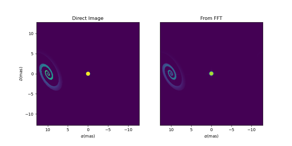
We create a model consisting of two components: The newly defined
oimSpiral class and a uniform disk (oimUD).
ud = oim.oimUD(d=2, f=0.2)
c = oimSpiral(dim=256, fwhm=5, P=0.1, width=0.2, pa=30, elong=2, x=10, f=0.8)
m = oim.oimModel(c, ud)
Then, we plot the image of the model (using the direct image formula and going back and forth to and from the Fourier plane).
fig, ax = plt.subplots(1, 2, figsize=(10, 5))
m.showModel(256, 0.1, swapAxes=True, fromFT=False,
            normPow=1, axe=ax[0], colorbar=False)
m.showModel(256, 0.1, swapAxes=True, fromFT=True,
            normPow=1, axe=ax[1], colorbar=False)
ax[1].get_yaxis().set_visible(False)
ax[0].set_title("Direct Image")
ax[1].set_title("From FFT")
And finally, the visibility from the models for a fixed wavelength and a series of baselines in two perpendicular orientations.
nB = 5000
nwl = 1
wl = 0.5e-6

B = np.linspace(0, 100, num=nB//2)
Bx = np.append(B, B*0)
By = np.append(B*0, B)

spfx = Bx/wl
spfy = By/wl

vc = m.getComplexCoherentFlux(spfx, spfy)
v = np.abs(vc/vc[0])

fig, ax = plt.subplots(1, 1)
label = ["East-West Baselines",]

ax.plot(B/wl/units.rad.to(units.mas),
        v[:nB//2], color="r", label="East-West Baselines")
ax.plot(B/wl/units.rad.to(units.mas),
        v[nB//2:], color="b", label="North-South Baselines")

ax.set_xlabel("B/$\lambda$ (cycles/mas)")
ax.set_ylabel("Visibility")
ax.legend()

Exp. Ring (Radial profile)
Note
Examples will be added when the oimComponentRadialProfile is implemented.
Creating New Interpolators
In the createCustomParamInterpolator.py
example we will create a new parameter interpolator derived from the
oimParaminterpolator class.
The new class will allow chromatic interpolation with a vector of evenly spaced values
in a range of wavelengths.
First we load some useful package and also set the random seed to a fixed value as we will use it to initalize our vector.
from pathlib import Path
from pprint import pprint

import matplotlib.colors as colors
import matplotlib.cm as cm
import matplotlib.pyplot as plt
import numpy as np
import oimodeler as oim
from scipy.interpolate import interp1d

np.random.seed(1)
As for the components, we derive our interpolator from a base class, this time
oimParamInterpolator.
We need to implement the, for this class unique oimParamInterpolator._init
method that will be called by the __init__ method of the base class.
This method should contain information on the interpolator parameters.
class oimParamLinearRangeWl(oim.oimParamInterpolator):
    def _init(self, param, wl0=2e-6, dwl=1e-9, values=[], kind="linear", **kwargs):

        self.kind = kind

        n = len(values)
        self.wl0 = (oim.oimParam(**oim._standardParameters["wl"]))
        self.wl0.name = "wl0"
        self.wl0.description = "Initial wl of the range"
        self.wl0.value = wl0
        self.wl0.free = False

        self.dwl = (oim.oimParam(**oim._standardParameters["wl"]))
        self.dwl.name = "dwl"
        self.dwl.description = "wl step in range"
        self.dwl.value = dwl
        self.dwl.free = False

        self.values = []

        for i in range(n):
            self.values.append(oim.oimParam(name=param.name, value=values[i],
                                            mini=param.min, maxi=param.max,
                                            description=param.description,
                                            unit=param.unit, free=param.free,
                                            error=param.error))
The first argument of the class, param is the
oimParam on which the new interpolator will be
built.
The next arguments are the interpolator parameters, here :
The initial wavelength of the range
wl0The wavelength step in the range of interpolation :
dwlThe values at the reference wavelength :
valuesThe method for interpolation (from scipy interp1d)
kind
The **kwargs is added for backward-compatibility.
The parameters wl0, dwl are created from the _standardParameters["wl"]
dictionary (contained in the oimParam module) for the
wavelength.
Their name, descriptions, and value are updated, and they are set as fixed parameter
by default (free=False).
The values vector of parameters is created from the input parameter param.
For each parameter in the vector the value is set to the proper one given as input
parameter.
The second method to implement is the
oimParamInterpolator._interpFunction
which is the core function of the interpolation. It has two input parameters: The
wavelength wl and the time t for which the parameter shoud be interpolated.
As our interoplator is not time dependent, we can ignore t.
def _interpFunction(self, wl, t):
    vals = np.array([vi.value for vi in self.values])
    nwl = vals.size
    wl0 = np.linspace(self.wl0.value, self.wl0.value +
                      self.dwl.value*nwl, num=nwl)
    return interp1d(wl0, vals, kind=self.kind, fill_value="extrapolate")(wl)
In this method we:
Create a numpy array from the values of the
self.valuesvector from theoimParamclass.A second numpy array for the regular grid of walvengths from the
self.wl0andself.dwlparameters.Interpolate the values at wl using the scipy interp1d function.
Return the resulting interpolated values of the parameter.
For model-fitting purposes, we also need to tell oimodeler what
are the parameters of our interpolator. This is done by implementing
the oimParamInterpolator._getParams
method. This method is called by a property params of
the base class oimParamInterpolator.
def _getParams(self):
    params = []
    params.extend(self.values)
    params.append(self.wl0)
    params.append(self.dwl)
    return params
This method simply returns the list of the interpolator parameters.
Here, the list of the reference values self.values, the initial wavelength self.wl0 and the wavelength step self.dwl. We omit the kind parameter as we consider it more as an option than a real parameter.
Finally, if we want to use our interpolator using the
oimInterp macro, we need to reference it
in the _interpolator dictionary contained in the oimParam
module.
oim._interpolator["rangeWl"] = oimParamLinearRangeWl
Now, we can use our new interpolator to build a component and a model.
Let’s build a chromatic uniform disk with 10 reference wavelengths between
2 and 2.5 microns. For the example, we will fill the values vector with
random diameters from 4 to 7 mas.
nref = 10
c = oim.oimUD(d=oim.oimInterp('rangeWl', wl0=2e-6, kind="cubic",
                              dwl=5e-8, values=np.random.rand(nref)*3+4))
m = oim.oimModel(c)
We can print the parameters of our model:
pprint(m.getParameters())
... {'c1_UD_x': oimParam at 0x17829999e80 : x=0 ± 0 mas range=[-inf,inf] free=False ,
     'c1_UD_y': oimParam at 0x17829999fd0 : y=0 ± 0 mas range=[-inf,inf] free=False ,
     'c1_UD_f': oimParam at 0x17829999f40 : f=1 ± 0  range=[-inf,inf] free=True ,
     'c1_UD_d_interp1': oimParam at 0x178253c9250 : d=5.251066014107722 ± 0 mas range=[-inf,inf] free=True ,
     'c1_UD_d_interp2': oimParam at 0x178253c9280 : d=6.160973480326474 ± 0 mas range=[-inf,inf] free=True ,
     'c1_UD_d_interp3': oimParam at 0x178253c92b0 : d=4.000343124452034 ± 0 mas range=[-inf,inf] free=True ,
     'c1_UD_d_interp4': oimParam at 0x178253c92e0 : d=4.9069977178955195 ± 0 mas range=[-inf,inf] free=True ,
     'c1_UD_d_interp5': oimParam at 0x178253c9310 : d=4.4402676724513395 ± 0 mas range=[-inf,inf] free=True ,
     'c1_UD_d_interp6': oimParam at 0x178253c9340 : d=4.277015784306394 ± 0 mas range=[-inf,inf] free=True ,
     'c1_UD_d_interp7': oimParam at 0x178253c9370 : d=4.558780634133012 ± 0 mas range=[-inf,inf] free=True ,
     'c1_UD_d_interp8': oimParam at 0x178253c93a0 : d=5.036682181129143 ± 0 mas range=[-inf,inf] free=True ,
     'c1_UD_d_interp9': oimParam at 0x178253c93d0 : d=5.19030242269201 ± 0 mas range=[-inf,inf] free=True ,
     'c1_UD_d_interp10': oimParam at 0x178253c9400 : d=5.616450202010071 ± 0 mas range=[-inf,inf] free=True ,
     'c1_UD_d_interp11': oimParam at 0x178253c9220 : wl0=2e-06 ± 0 m range=[0,inf] free=False ,
     'c1_UD_d_interp12': oimParam at 0x178253b5df0 : dwl=5e-08 ± 0 m range=[0,inf] free=False }
The interpolator replaced the single oimParam
for the diameter c1_UD_d by 12 oimParam:
10 for the reference values of the diameter (filled by random in our initialization),
one for the initial wavelength wl0 and another for the wavèlength step dwl.
We can also get the free parameters:
pprint(m.getFreeParameters())
... {'c1_UD_f': oimParam at 0x17829999f40 : f=1 ± 0  range=[-inf,inf] free=True ,
     'c1_UD_d_interp1': oimParam at 0x178253c9250 : d=5.251066014107722 ± 0 mas range=[-inf,inf] free=True ,
     'c1_UD_d_interp2': oimParam at 0x178253c9280 : d=6.160973480326474 ± 0 mas range=[-inf,inf] free=True ,
     'c1_UD_d_interp3': oimParam at 0x178253c92b0 : d=4.000343124452034 ± 0 mas range=[-inf,inf] free=True ,
     'c1_UD_d_interp4': oimParam at 0x178253c92e0 : d=4.9069977178955195 ± 0 mas range=[-inf,inf] free=True ,
     'c1_UD_d_interp5': oimParam at 0x178253c9310 : d=4.4402676724513395 ± 0 mas range=[-inf,inf] free=True ,
     'c1_UD_d_interp6': oimParam at 0x178253c9340 : d=4.277015784306394 ± 0 mas range=[-inf,inf] free=True ,
     'c1_UD_d_interp7': oimParam at 0x178253c9370 : d=4.558780634133012 ± 0 mas range=[-inf,inf] free=True ,
     'c1_UD_d_interp8': oimParam at 0x178253c93a0 : d=5.036682181129143 ± 0 mas range=[-inf,inf] free=True ,
     'c1_UD_d_interp9': oimParam at 0x178253c93d0 : d=5.19030242269201 ± 0 mas range=[-inf,inf] free=True ,
     'c1_UD_d_interp10': oimParam at 0x178253c9400 : d=5.616450202010071 ± 0 mas range=[-inf,inf] free=True }
Here the x and y parameters are removed as they are fixed by default,
as well as wl0 and dwl.
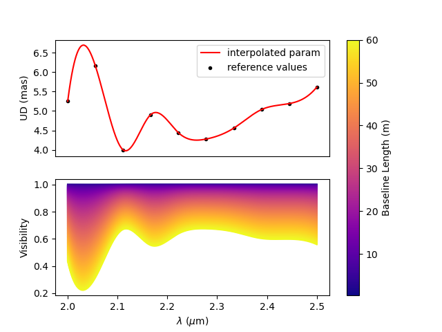
Let’s plot the interpolated values of the parameters in the 2-2.5 micron range with 1000 values as well as the corresponding visibility for 200 East-West baselines ranging from 0 to 60m.
First, we create the wavelength vector and the spatial frequencies and wavelength arrays.
nB = 200
B = np.linspace(0, 60, num=nB)
nwl = 1000
wl = np.linspace(2.0e-6, 2.5e-6, num=nwl)
Bx_arr = np.tile(B[None, :], (nwl, 1)).flatten()
wl_arr = np.tile(wl[:, None], (1, nB)).flatten()
spfx_arr = Bx_arr/wl_arr
spfy_arr = spfx_arr*0
Finally, we compute the visibilty using the
oimModel.getComplexCoherentFlux method
and plot everything together.
v = np.abs(m.getComplexCoherentFlux(spfx_arr, spfy_arr, wl_arr).reshape(nwl, nB))

fig, ax = plt.subplots(2, 1)
ax[0].plot(wl*1e6, c.params['d'](wl, 0), color="r", label="interpolated param")
ax[0].scatter(wl0*1e6, vals, marker=".", color="k", label="reference values")
ax[0].set_ylabel("UD (mas)")
ax[0].get_xaxis().set_visible(False)
ax[0].legend()

for iB in range(1,nB):
    ax[1].plot(wl*1e6, v[:, iB]/v[:, 0], color=plt.cm.plasma(iB/(nB-1)))

ax[1].set_xlabel("$\lambda$ ($\mu$m)")
ax[1].set_ylabel("Visibility")

norm = colors.Normalize(vmin=np.min(B[1:]), vmax=np.max(B))
sm = cm.ScalarMappable(cmap=plt.cm.plasma, norm=norm)
fig.colorbar(sm, ax=ax, label="Baseline Length (m)")